Pre-stack modelling

This example shows how to create pre-stack angle gathers using the pylops.avo.prestack.PrestackLinearModelling operator.

import matplotlib.pyplot as plt
import numpy as np
from scipy.signal import filtfilt

import pylops
from pylops.utils.wavelets import ricker

plt.close("all")
np.random.seed(0)

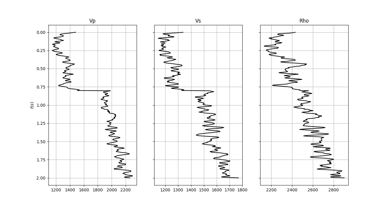
Let’s start by creating the input elastic property profiles and wavelet

nt0 = 501
dt0 = 0.004
ntheta = 21

t0 = np.arange(nt0) * dt0
thetamin, thetamax = 0, 40
theta = np.linspace(thetamin, thetamax, ntheta)

# Elastic property profiles
vp = (
    1200 + np.arange(nt0) + filtfilt(np.ones(5) / 5.0, 1, np.random.normal(0, 160, nt0))
)
vs = 600 + vp / 2 + filtfilt(np.ones(5) / 5.0, 1, np.random.normal(0, 100, nt0))
rho = 1000 + vp + filtfilt(np.ones(5) / 5.0, 1, np.random.normal(0, 120, nt0))
vp[201:] += 500
vs[201:] += 200
rho[201:] += 100

# Wavelet
ntwav = 81
wav, twav, wavc = ricker(t0[: ntwav // 2 + 1], 5)

# vs/vp profile
vsvp = 0.5
vsvp_z = np.linspace(0.4, 0.6, nt0)

# Model
m = np.stack((np.log(vp), np.log(vs), np.log(rho)), axis=1)

fig, axs = plt.subplots(1, 3, figsize=(13, 7), sharey=True)
axs[0].plot(vp, t0, "k")
axs[0].set_title("Vp")
axs[0].set_ylabel(r"$t(s)$")
axs[0].invert_yaxis()
axs[0].grid()
axs[1].plot(vs, t0, "k")
axs[1].set_title("Vs")
axs[1].invert_yaxis()
axs[1].grid()
axs[2].plot(rho, t0, "k")
axs[2].set_title("Rho")
axs[2].invert_yaxis()
axs[2].grid()

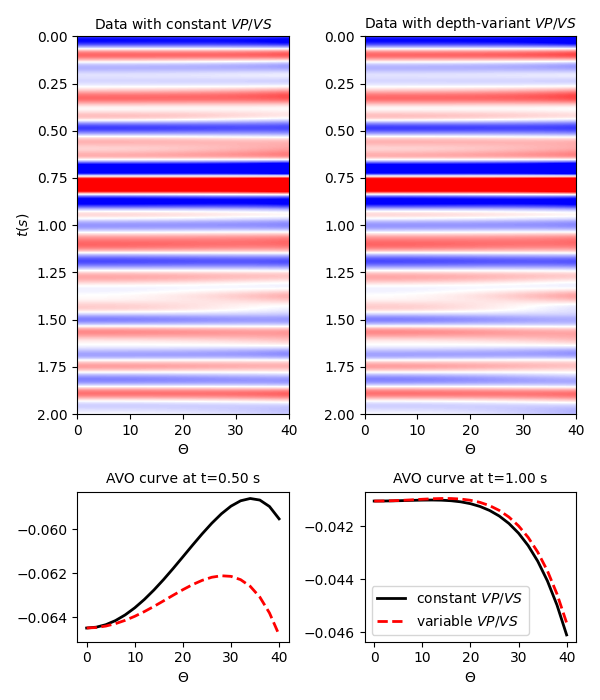
We create now the operators to model a synthetic pre-stack seismic gather with a zero-phase using both a constant and a depth-variant vsvp profile

# constant vsvp
PPop_const = pylops.avo.prestack.PrestackLinearModelling(
    wav, theta, vsvp=vsvp, nt0=nt0, linearization="akirich"
)

# depth-variant vsvp
PPop_variant = pylops.avo.prestack.PrestackLinearModelling(
    wav, theta, vsvp=vsvp_z, linearization="akirich"
)

Let’s apply those operators to the elastic model and create some synthetic data

dPP_const = PPop_const * m.ravel()
dPP_const = dPP_const.reshape(nt0, ntheta)

dPP_variant = PPop_variant * m.ravel()
dPP_variant = dPP_variant.reshape(nt0, ntheta)

Finally we visualize the two datasets

# sphinx_gallery_thumbnail_number = 2
fig = plt.figure(figsize=(6, 7))
ax1 = plt.subplot2grid((3, 2), (0, 0), rowspan=2)
ax2 = plt.subplot2grid((3, 2), (0, 1), rowspan=2)
ax3 = plt.subplot2grid((3, 2), (2, 0))
ax4 = plt.subplot2grid((3, 2), (2, 1))
ax1.imshow(
    dPP_const,
    cmap="bwr",
    extent=(theta[0], theta[-1], t0[-1], t0[0]),
    vmin=-0.1,
    vmax=0.1,
)
ax1.set_xlabel(r"$\Theta$")
ax1.set_ylabel(r"$t(s)$")
ax1.set_title(r"Data with constant $VP/VS$", fontsize=10)
ax1.axis("tight")
ax2.imshow(
    dPP_variant,
    cmap="bwr",
    extent=(theta[0], theta[-1], t0[-1], t0[0]),
    vmin=-0.1,
    vmax=0.1,
)
ax2.set_title(r"Data with depth-variant $VP/VS$", fontsize=10)
ax2.set_xlabel(r"$\Theta$")
ax2.axis("tight")
ax3.plot(theta, dPP_const[nt0 // 4], "k", lw=2)
ax3.plot(theta, dPP_variant[nt0 // 4], "--r", lw=2)
ax3.set_title("AVO curve at t=%.2f s" % t0[nt0 // 4], fontsize=10)
ax3.set_xlabel(r"$\Theta$")
ax4.plot(theta, dPP_const[nt0 // 2], "k", lw=2, label=r"constant $VP/VS$")
ax4.plot(theta, dPP_variant[nt0 // 2], "--r", lw=2, label=r"variable $VP/VS$")
ax4.set_title("AVO curve at t=%.2f s" % t0[nt0 // 2], fontsize=10)
ax4.set_xlabel(r"$\Theta$")
ax4.legend()
plt.tight_layout()