Note
Click here to download the full example code
Causal Integration
This example shows how to use the pylops.CausalIntegration
operator to integrate an input signal (in forward mode) and to apply a smooth,
regularized derivative (in inverse mode). This is a very interesting
by-product of this operator which may result very useful when the data
to which you want to apply a numerical derivative is noisy.
import matplotlib.pyplot as plt
import numpy as np

import pylops

plt.close("all")
Let’s start with a 1D example. Define the input parameters: number of samples
of input signal (nt), sampling step (dt) as well as the input
signal which will be equal to \(x(t)=\sin(t)\):
We can now create our causal integration operator and apply it to the input
signal. We can also compute the analytical integral
\(y(t)=\int \sin(t)\,\mathrm{d}t=-\cos(t)\) and compare the results. We can also
invert the integration operator and by remembering that this is equivalent
to a first order derivative, we will compare our inverted model with the
result obtained by simply applying the pylops.FirstDerivative
forward operator to the same data.
Note that, as explained in details in pylops.CausalIntegration,
integration has no unique solution, as any constant \(c\) can be added
to the integrated signal \(y\), for example if \(x(t)=t^2\) the
\(y(t) = \int t^2 \,\mathrm{d}t = \frac{t^3}{3} + c\). We thus subtract first
sample from the analytical integral to obtain the same result as the
numerical one.
Cop = pylops.CausalIntegration(nt, sampling=dt, halfcurrent=True)
yana = -np.cos(t) + np.cos(t[0])
y = Cop * x
xinv = Cop / y
# Numerical derivative
Dop = pylops.FirstDerivative(nt, sampling=dt)
xder = Dop * y
# Visualize data and inversion
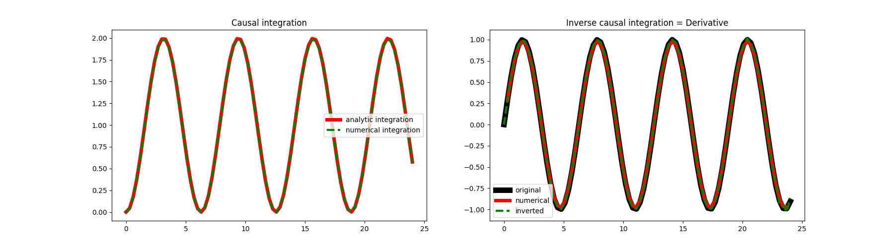
fig, axs = plt.subplots(1, 2, figsize=(18, 5))
axs[0].plot(t, yana, "r", lw=5, label="analytic integration")
axs[0].plot(t, y, "--g", lw=3, label="numerical integration")
axs[0].legend()
axs[0].set_title("Causal integration")
axs[1].plot(t, x, "k", lw=8, label="original")
axs[1].plot(t[1:-1], xder[1:-1], "r", lw=5, label="numerical")
axs[1].plot(t, xinv, "--g", lw=3, label="inverted")
axs[1].legend()
axs[1].set_title("Inverse causal integration = Derivative")
Out:
Text(0.5, 1.0, 'Inverse causal integration = Derivative')
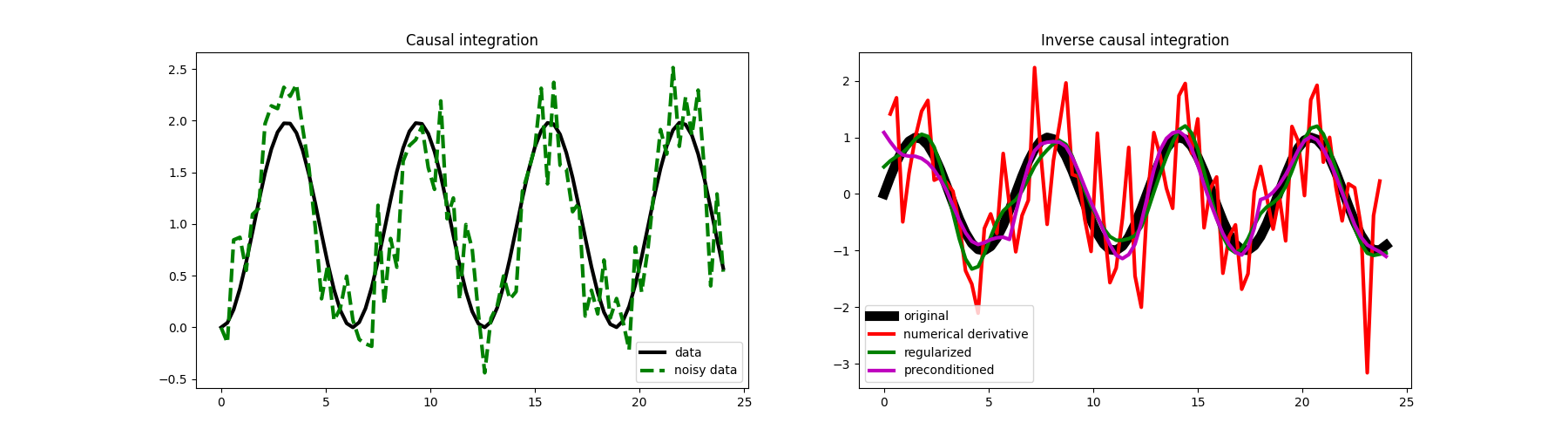
As expected we obtain the same result. Let’s see what happens if we now add some random noise to our data.
# Add noise
yn = y + np.random.normal(0, 4e-1, y.shape)

# Numerical derivative
Dop = pylops.FirstDerivative(nt, sampling=dt)
xder = Dop * yn

# Regularized derivative
Rop = pylops.SecondDerivative(nt)
xreg = pylops.RegularizedInversion(
    Cop, [Rop], yn, epsRs=[1e0], **dict(iter_lim=100, atol=1e-5)
)

# Preconditioned derivative
Sop = pylops.Smoothing1D(41, nt)
xp = pylops.PreconditionedInversion(Cop, Sop, yn, **dict(iter_lim=10, atol=1e-3))

# Visualize data and inversion
fig, axs = plt.subplots(1, 2, figsize=(18, 5))
axs[0].plot(t, y, "k", lw=3, label="data")
axs[0].plot(t, yn, "--g", lw=3, label="noisy data")
axs[0].legend()
axs[0].set_title("Causal integration")
axs[1].plot(t, x, "k", lw=8, label="original")
axs[1].plot(t[1:-1], xder[1:-1], "r", lw=3, label="numerical derivative")
axs[1].plot(t, xreg, "g", lw=3, label="regularized")
axs[1].plot(t, xp, "m", lw=3, label="preconditioned")
axs[1].legend()
axs[1].set_title("Inverse causal integration")
Out:
Text(0.5, 1.0, 'Inverse causal integration')
We can see here the great advantage of framing our numerical derivative as an inverse problem, and more specifically as the inverse of the causal integration operator.
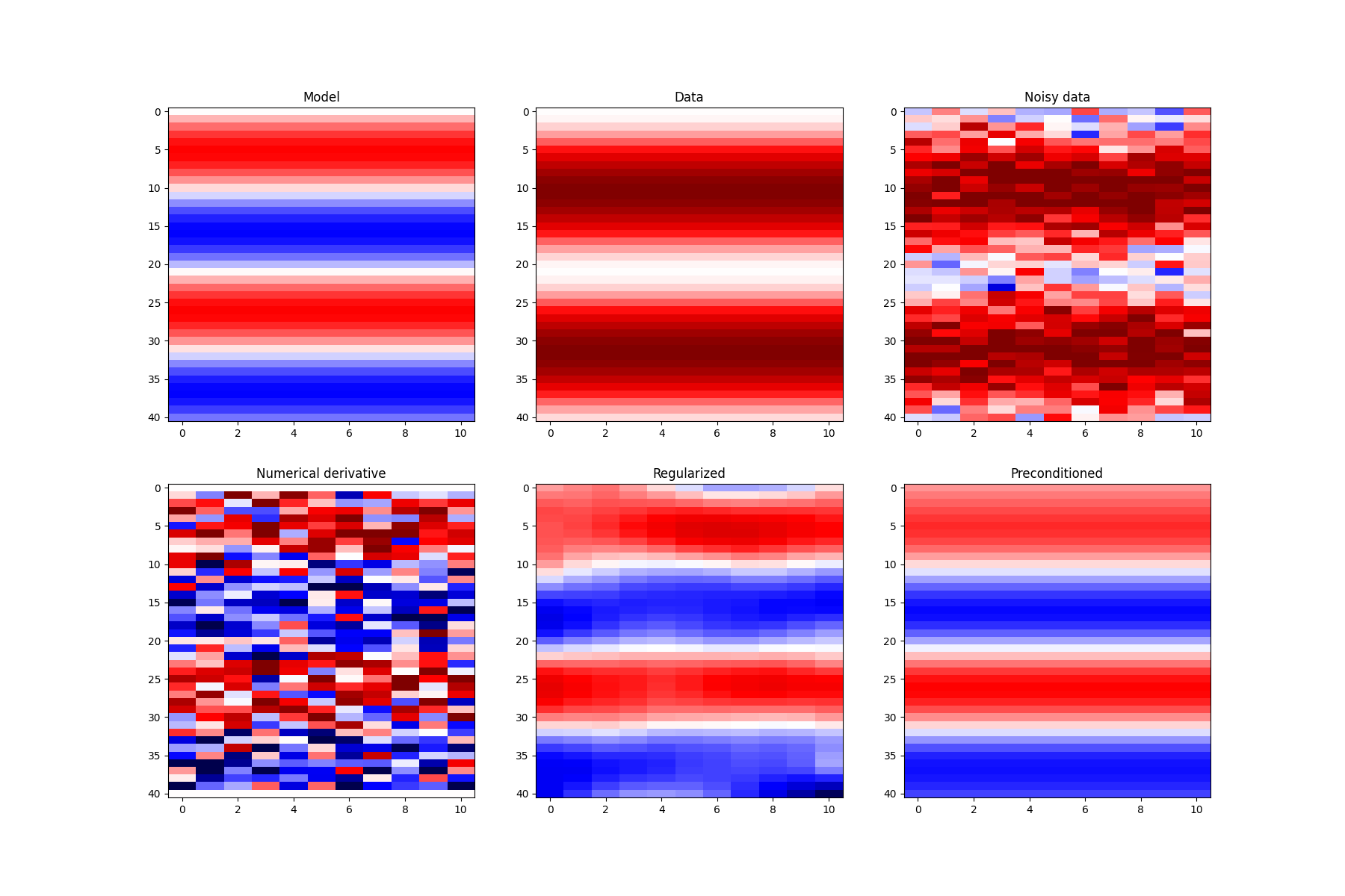
Let’s conclude with a 2d example where again the integration/derivative will be performed along the first axis
nt, nx = 41, 11
dt = 0.3
ot = 0
t = np.arange(nt) * dt + ot
x = np.outer(np.sin(t), np.ones(nx))
Cop = pylops.CausalIntegration(
nt * nx, dims=(nt, nx), sampling=dt, dir=0, halfcurrent=True
)
y = Cop * x.ravel()
y = y.reshape(nt, nx)
yn = y + np.random.normal(0, 4e-1, y.shape)
# Numerical derivative
Dop = pylops.FirstDerivative(nt * nx, dims=(nt, nx), dir=0, sampling=dt)
xder = Dop * yn.ravel()
xder = xder.reshape(nt, nx)
# Regularized derivative
Rop = pylops.Laplacian(dims=(nt, nx))
xreg = pylops.RegularizedInversion(
Cop, [Rop], yn.ravel(), epsRs=[1e0], **dict(iter_lim=100, atol=1e-5)
)
xreg = xreg.reshape(nt, nx)
# Preconditioned derivative
Sop = pylops.Smoothing2D((11, 21), dims=(nt, nx))
xp = pylops.PreconditionedInversion(
Cop, Sop, yn.ravel(), **dict(iter_lim=10, atol=1e-2)
)
xp = xp.reshape(nt, nx)
# Visualize data and inversion
vmax = 2 * np.max(np.abs(x))
fig, axs = plt.subplots(2, 3, figsize=(18, 12))
axs[0][0].imshow(x, cmap="seismic", vmin=-vmax, vmax=vmax)
axs[0][0].set_title("Model")
axs[0][0].axis("tight")
axs[0][1].imshow(y, cmap="seismic", vmin=-vmax, vmax=vmax)
axs[0][1].set_title("Data")
axs[0][1].axis("tight")
axs[0][2].imshow(yn, cmap="seismic", vmin=-vmax, vmax=vmax)
axs[0][2].set_title("Noisy data")
axs[0][2].axis("tight")
axs[1][0].imshow(xder, cmap="seismic", vmin=-vmax, vmax=vmax)
axs[1][0].set_title("Numerical derivative")
axs[1][0].axis("tight")
axs[1][1].imshow(xreg, cmap="seismic", vmin=-vmax, vmax=vmax)
axs[1][1].set_title("Regularized")
axs[1][1].axis("tight")
axs[1][2].imshow(xp, cmap="seismic", vmin=-vmax, vmax=vmax)
axs[1][2].set_title("Preconditioned")
axs[1][2].axis("tight")
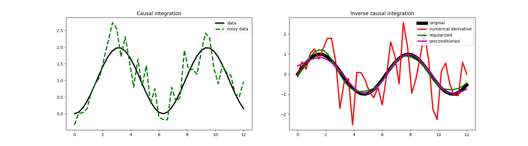
# Visualize data and inversion at a chosen xlocation
fig, axs = plt.subplots(1, 2, figsize=(18, 5))
axs[0].plot(t, y[:, nx // 2], "k", lw=3, label="data")
axs[0].plot(t, yn[:, nx // 2], "--g", lw=3, label="noisy data")
axs[0].legend()
axs[0].set_title("Causal integration")
axs[1].plot(t, x[:, nx // 2], "k", lw=8, label="original")
axs[1].plot(t, xder[:, nx // 2], "r", lw=3, label="numerical derivative")
axs[1].plot(t, xreg[:, nx // 2], "g", lw=3, label="regularized")
axs[1].plot(t, xp[:, nx // 2], "m", lw=3, label="preconditioned")
axs[1].legend()
axs[1].set_title("Inverse causal integration")
Out:
Text(0.5, 1.0, 'Inverse causal integration')
Total running time of the script: ( 0 minutes 1.504 seconds)