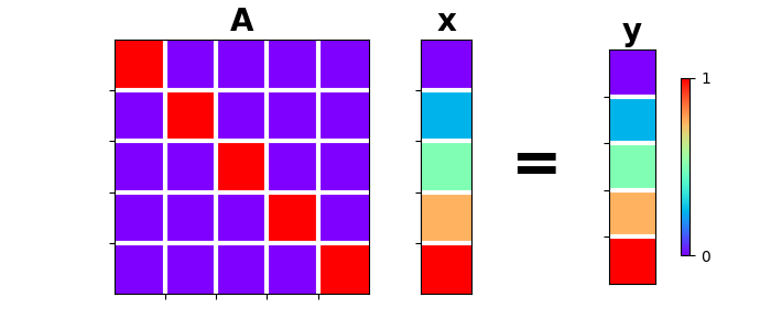
Identity

This example shows how to use the pylops.Identity operator to transfer model into data and viceversa.

import matplotlib.gridspec as pltgs
import matplotlib.pyplot as plt
import numpy as np

import pylops

plt.close("all")

Let’s define an identity operator \(\mathbf{Iop}\) with same number of elements for data and model (\(N=M\)).

N, M = 5, 5
x = np.arange(M)
Iop = pylops.Identity(M, dtype="int")

y = Iop * x
xadj = Iop.H * y

gs = pltgs.GridSpec(1, 6)
fig = plt.figure(figsize=(7, 3))
ax = plt.subplot(gs[0, 0:3])
im = ax.imshow(np.eye(N), cmap="rainbow")
ax.set_title("A", size=20, fontweight="bold")
ax.set_xticks(np.arange(N - 1) + 0.5)
ax.set_yticks(np.arange(M - 1) + 0.5)
ax.grid(linewidth=3, color="white")
ax.xaxis.set_ticklabels([])
ax.yaxis.set_ticklabels([])
ax = plt.subplot(gs[0, 3])
ax.imshow(x[:, np.newaxis], cmap="rainbow")
ax.set_title("x", size=20, fontweight="bold")
ax.set_xticks([])
ax.set_yticks(np.arange(M - 1) + 0.5)
ax.grid(linewidth=3, color="white")
ax.xaxis.set_ticklabels([])
ax.yaxis.set_ticklabels([])
ax = plt.subplot(gs[0, 4])
ax.text(
    0.35,
    0.5,
    "=",
    horizontalalignment="center",
    verticalalignment="center",
    size=40,
    fontweight="bold",
)
ax.axis("off")
ax = plt.subplot(gs[0, 5])
ax.imshow(y[:, np.newaxis], cmap="rainbow")
ax.set_title("y", size=20, fontweight="bold")
ax.set_xticks([])
ax.set_yticks(np.arange(N - 1) + 0.5)
ax.grid(linewidth=3, color="white")
ax.xaxis.set_ticklabels([])
ax.yaxis.set_ticklabels([])
fig.colorbar(im, ax=ax, ticks=[0, 1], pad=0.3, shrink=0.7)

Out:

<matplotlib.colorbar.Colorbar object at 0x7f90d0a10b38>

Similarly we can consider the case with data bigger than model

N, M = 10, 5
x = np.arange(M)
Iop = pylops.Identity(N, M, dtype="int")

y = Iop * x
xadj = Iop.H * y

print("x = %s " % x)
print("I*x = %s " % y)
print("I'*y = %s " % xadj)

Out:

x = [0 1 2 3 4]
I*x = [0 1 2 3 4 0 0 0 0 0]
I'*y = [0 1 2 3 4]

and model bigger than data

N, M = 5, 10
x = np.arange(M)
Iop = pylops.Identity(N, M, dtype="int")

y = Iop * x
xadj = Iop.H * y

print("x = %s " % x)
print("I*x = %s " % y)
print("I'*y = %s " % xadj)

Out:

x = [0 1 2 3 4 5 6 7 8 9]
I*x = [0 1 2 3 4]
I'*y = [0 1 2 3 4 0 0 0 0 0]

Note that this operator can be useful in many real-life applications when for example we want to manipulate a subset of the model array and keep intact the rest of the array. For example:

\[\begin{split}\begin{bmatrix} \mathbf{A} \quad \mathbf{I} \end{bmatrix} \begin{bmatrix} \mathbf{x_1} \\ \mathbf{x_2} \end{bmatrix} = \mathbf{A} \mathbf{x_1} + \mathbf{x_2}\end{split}\]

Refer to the tutorial on Optimization for more details on this.