Note
Click here to download the full example code
Linear Regression
This example shows how to use the pylops.LinearRegression operator
to perform Linear regression analysis.
In short, linear regression is the problem of finding the best fitting coefficients, namely intercept \(\mathbf{x_0}\) and gradient \(\mathbf{x_1}\), for this equation:
\[y_i = x_0 + x_1 t_i \qquad \forall i=0,1,\ldots,N-1\]
As we can express this problem in a matrix form:
\[\mathbf{y}= \mathbf{A} \mathbf{x}\]
our solution can be obtained by solving the following optimization problem:
\[J= \|\mathbf{y} - \mathbf{A} \mathbf{x}\|_2\]
See documentation of pylops.LinearRegression for more detailed
definition of the forward problem.
import matplotlib.pyplot as plt
import numpy as np

import pylops

plt.close("all")
np.random.seed(10)
Define the input parameters: number of samples along the t-axis (N),
linear regression coefficients (x), and standard deviation of noise
to be added to data (sigma).
Let’s create the time axis and initialize the
pylops.LinearRegression operator
We can then apply the operator in forward mode to compute our data points
along the x-axis (y). We will also generate some random gaussian noise
and create a noisy version of the data (yn).
We are now ready to solve our problem. As we are using an operator from the
pylops.LinearOperator family, we can simply use /,
which in this case will solve the system by means of an iterative solver
(i.e., scipy.sparse.linalg.lsqr).
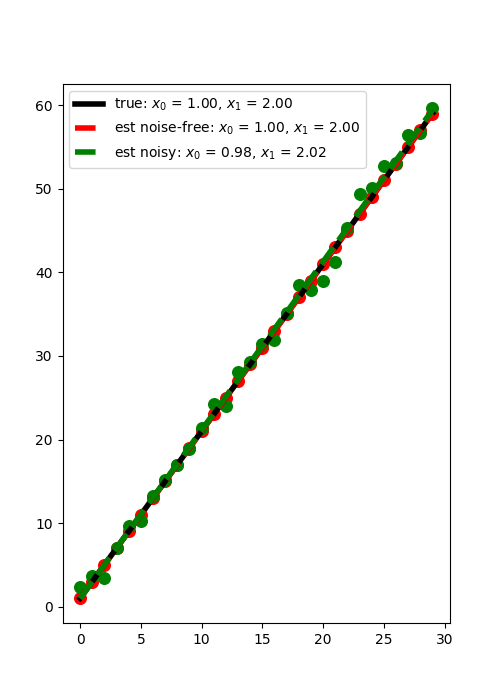
Let’s plot the best fitting line for the case of noise free and noisy data
plt.figure(figsize=(5, 7))
plt.plot(
    np.array([t.min(), t.max()]),
    np.array([t.min(), t.max()]) * x[1] + x[0],
    "k",
    lw=4,
    label=r"true: $x_0$ = %.2f, $x_1$ = %.2f" % (x[0], x[1]),
)
plt.plot(
    np.array([t.min(), t.max()]),
    np.array([t.min(), t.max()]) * xest[1] + xest[0],
    "--r",
    lw=4,
    label=r"est noise-free: $x_0$ = %.2f, $x_1$ = %.2f" % (xest[0], xest[1]),
)
plt.plot(
    np.array([t.min(), t.max()]),
    np.array([t.min(), t.max()]) * xnest[1] + xnest[0],
    "--g",
    lw=4,
    label=r"est noisy: $x_0$ = %.2f, $x_1$ = %.2f" % (xnest[0], xnest[1]),
)
plt.scatter(t, y, c="r", s=70)
plt.scatter(t, yn, c="g", s=70)
plt.legend()
Out:
<matplotlib.legend.Legend object at 0x7f90d01f4518>
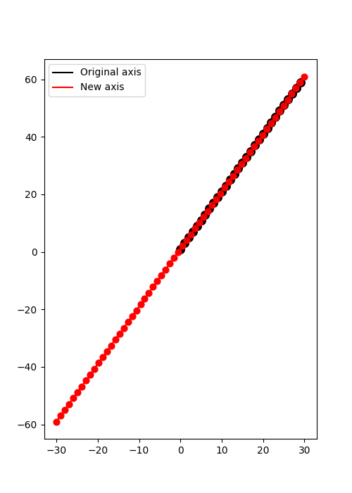
Once that we have estimated the best fitting coefficients \(\mathbf{x}\) we can now use them to compute the y values for a different set of values along the t-axis.
t1 = np.linspace(-N, N, 2 * N, dtype="float64")
y1 = LRop.apply(t1, xest)

plt.figure(figsize=(5, 7))
plt.plot(t, y, "k", label="Original axis")
plt.plot(t1, y1, "r", label="New axis")
plt.scatter(t, y, c="k", s=70)
plt.scatter(t1, y1, c="r", s=40)
plt.legend()
Out:
<matplotlib.legend.Legend object at 0x7f90d1272da0>
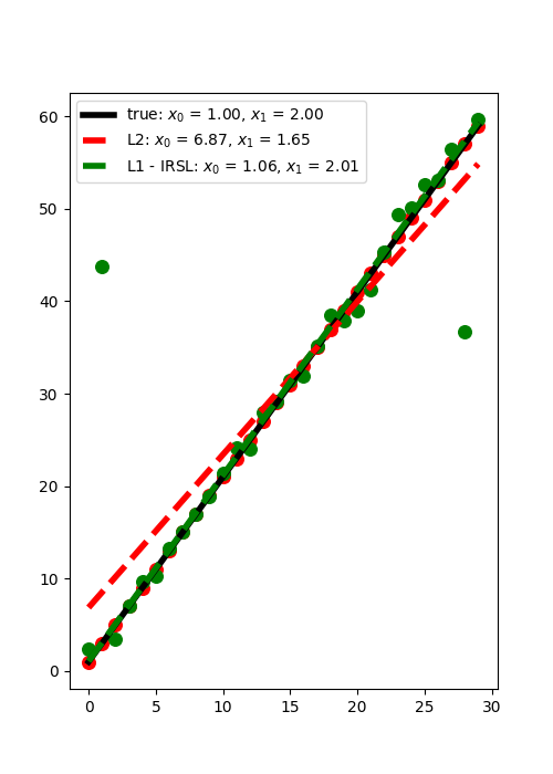
We consider now the case where some of the observations have large errors.
Such elements are generally referred to as outliers and can affect the
quality of the least-squares solution if not treated with care. In this
example we will see how using a L1 solver such as
pylops.optimization.sparsity.IRLS can drammatically improve the
quality of the estimation of intercept and gradient.
# Add outliers
yn[1] += 40
yn[N - 2] -= 20

# IRLS
nouter = 20
epsR = 1e-2
epsI = 0
tolIRLS = 1e-2

xnest = LRop / yn
xirls, nouter, xirls_hist, rw_hist = pylops.optimization.sparsity.IRLS(
    LRop,
    yn,
    nouter,
    threshR=False,
    epsR=epsR,
    epsI=epsI,
    tolIRLS=tolIRLS,
    returnhistory=True,
)
print("IRLS converged at %d iterations..." % nouter)

plt.figure(figsize=(5, 7))
plt.plot(
    np.array([t.min(), t.max()]),
    np.array([t.min(), t.max()]) * x[1] + x[0],
    "k",
    lw=4,
    label=r"true: $x_0$ = %.2f, $x_1$ = %.2f" % (x[0], x[1]),
)
plt.plot(
    np.array([t.min(), t.max()]),
    np.array([t.min(), t.max()]) * xnest[1] + xnest[0],
    "--r",
    lw=4,
    label=r"L2: $x_0$ = %.2f, $x_1$ = %.2f" % (xnest[0], xnest[1]),
)
plt.plot(
    np.array([t.min(), t.max()]),
    np.array([t.min(), t.max()]) * xirls[1] + xirls[0],
    "--g",
    lw=4,
    label=r"L1 - IRSL: $x_0$ = %.2f, $x_1$ = %.2f" % (xirls[0], xirls[1]),
)
plt.scatter(t, y, c="r", s=70)
plt.scatter(t, yn, c="g", s=70)
plt.legend()
Out:
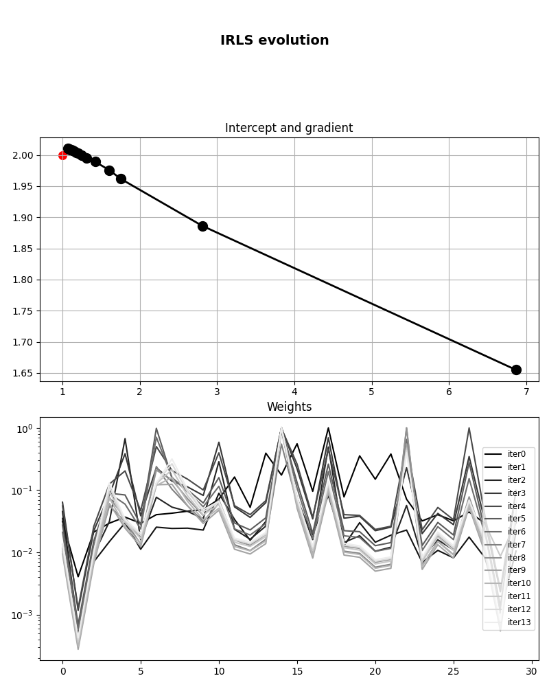
IRLS converged at 14 iterations...

<matplotlib.legend.Legend object at 0x7f90d0c6d588>
Let’s finally take a look at the convergence of IRLS. First we visualize the evolution of intercept and gradient
fig, axs = plt.subplots(2, 1, figsize=(8, 10))
fig.suptitle("IRLS evolution", fontsize=14, fontweight="bold", y=0.95)
axs[0].plot(xirls_hist[:, 0], xirls_hist[:, 1], ".-k", lw=2, ms=20)
axs[0].scatter(x[0], x[1], c="r", s=70)
axs[0].set_title("Intercept and gradient")
axs[0].grid()
for iiter in range(nouter):
    axs[1].semilogy(
        rw_hist[iiter],
        color=(iiter / nouter, iiter / nouter, iiter / nouter),
        label="iter%d" % iiter,
    )
axs[1].set_title("Weights")
axs[1].legend(loc=5, fontsize="small")
plt.tight_layout()
plt.subplots_adjust(top=0.8)
Total running time of the script: ( 0 minutes 1.066 seconds)