Pre-stack modelling

This example shows how to create pre-stack angle gathers using the pylops.avo.prestack.PrestackLinearModelling operator.

import matplotlib.pyplot as plt
import numpy as np
from mpl_toolkits.axes_grid1.axes_divider import make_axes_locatable
from scipy.signal import filtfilt

import pylops
from pylops.utils.wavelets import ricker

plt.close("all")
np.random.seed(0)

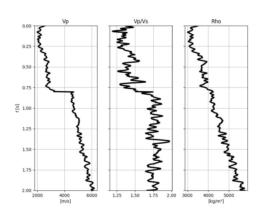
Let’s start by creating the input elastic property profiles and wavelet

nt0 = 501
dt0 = 0.004
ntheta = 21

t0 = np.arange(nt0) * dt0
thetamin, thetamax = 0, 40
theta = np.linspace(thetamin, thetamax, ntheta)

# Elastic property profiles
vp = (
    2000
    + 5 * np.arange(nt0)
    + 2 * filtfilt(np.ones(5) / 5.0, 1, np.random.normal(0, 160, nt0))
)
vs = 600 + vp / 2 + 3 * filtfilt(np.ones(5) / 5.0, 1, np.random.normal(0, 100, nt0))
rho = 1000 + vp + filtfilt(np.ones(5) / 5.0, 1, np.random.normal(0, 120, nt0))
vp[201:] += 1500
vs[201:] += 500
rho[201:] += 100

# Wavelet
ntwav = 81
wav, twav, wavc = ricker(t0[: ntwav // 2 + 1], 5)

# vs/vp profile
vsvp = 0.5
vsvp_z = vs / vp

# Model
m = np.stack((np.log(vp), np.log(vs), np.log(rho)), axis=1)

fig, axs = plt.subplots(1, 3, figsize=(9, 7), sharey=True)
axs[0].plot(vp, t0, "k", lw=3)
axs[0].set(xlabel="[m/s]", ylabel=r"$t$ [s]", ylim=[t0[0], t0[-1]], title="Vp")
axs[0].grid()
axs[1].plot(vp / vs, t0, "k", lw=3)
axs[1].set(title="Vp/Vs")
axs[1].grid()
axs[2].plot(rho, t0, "k", lw=3)
axs[2].set(xlabel="[kg/m³]", title="Rho")
axs[2].invert_yaxis()
axs[2].grid()

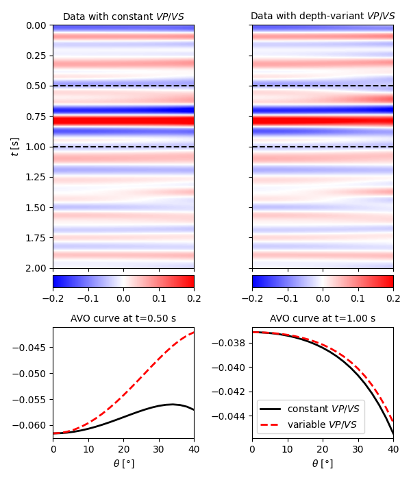
We create now the operators to model a synthetic pre-stack seismic gather with a zero-phase using both a constant and a depth-variant vsvp profile

# constant vsvp
PPop_const = pylops.avo.prestack.PrestackLinearModelling(
    wav, theta, vsvp=vsvp, nt0=nt0, linearization="akirich"
)

# depth-variant vsvp
PPop_variant = pylops.avo.prestack.PrestackLinearModelling(
    wav, theta, vsvp=vsvp_z, linearization="akirich"
)

Let’s apply those operators to the elastic model and create some synthetic data

dPP_const = PPop_const * m
dPP_variant = PPop_variant * m

Finally we visualize the two datasets

# sphinx_gallery_thumbnail_number = 2
fig = plt.figure(figsize=(6, 7))
ax1 = plt.subplot2grid((3, 2), (0, 0), rowspan=2)
ax2 = plt.subplot2grid((3, 2), (0, 1), rowspan=2, sharey=ax1)
ax3 = plt.subplot2grid((3, 2), (2, 0), sharex=ax1)
ax4 = plt.subplot2grid((3, 2), (2, 1), sharex=ax2)
im = ax1.imshow(
    dPP_const,
    cmap="bwr",
    extent=(theta[0], theta[-1], t0[-1], t0[0]),
    vmin=-0.2,
    vmax=0.2,
)
cax = make_axes_locatable(ax1).append_axes("bottom", size="5%", pad="3%")
cb = fig.colorbar(im, cax=cax, orientation="horizontal")
cb.ax.xaxis.set_ticks_position("bottom")
ax1.set(ylabel=r"$t$ [s]")
ax1.set_title(r"Data with constant $VP/VS$", fontsize=10)
ax1.tick_params(labelbottom=False)
ax1.axhline(t0[nt0 // 4], color="k", linestyle="--")
ax1.axhline(t0[nt0 // 2], color="k", linestyle="--")
ax1.axis("tight")

im = ax2.imshow(
    dPP_variant,
    cmap="bwr",
    extent=(theta[0], theta[-1], t0[-1], t0[0]),
    vmin=-0.2,
    vmax=0.2,
)
cax = make_axes_locatable(ax2).append_axes("bottom", size="5%", pad="3%")
cb = fig.colorbar(im, cax=cax, orientation="horizontal")
cb.ax.xaxis.set_ticks_position("bottom")
ax2.set_title(r"Data with depth-variant $VP/VS$", fontsize=10)
ax2.tick_params(labelbottom=False, labelleft=False)
ax2.axhline(t0[nt0 // 4], color="k", linestyle="--")
ax2.axhline(t0[nt0 // 2], color="k", linestyle="--")
ax2.axis("tight")

ax3.plot(theta, dPP_const[nt0 // 4], "k", lw=2)
ax3.plot(theta, dPP_variant[nt0 // 4], "--r", lw=2)
ax3.set(xlabel=r"$\theta$ [°]")
ax3.set_title("AVO curve at t=%.2f s" % t0[nt0 // 4], fontsize=10)
ax4.plot(theta, dPP_const[nt0 // 2], "k", lw=2, label=r"constant $VP/VS$")
ax4.plot(theta, dPP_variant[nt0 // 2], "--r", lw=2, label=r"variable $VP/VS$")
ax4.set(xlabel=r"$\theta$ [°]")
ax4.set_title("AVO curve at t=%.2f s" % t0[nt0 // 2], fontsize=10)
ax4.legend()
plt.tight_layout()