Patching

This example shows how to use the pylops.signalprocessing.Patch2D and pylops.signalprocessing.Patch3D operators to perform repeated transforms over small patches of a 2-dimensional or 3-dimensional array. The transforms that we apply in this example are the pylops.signalprocessing.FFT2D and pylops.signalprocessing.FFT3D but this operator has been designed to allow a variety of transforms as long as they operate with signals that are 2- or 3-dimensional in nature, respectively.

import matplotlib.pyplot as plt
import numpy as np

import pylops

plt.close("all")

Let’s start by creating an 2-dimensional array of size \(n_x \times n_t\) composed of 3 parabolic events

par = {"ox": -140, "dx": 2, "nx": 140, "ot": 0, "dt": 0.004, "nt": 200, "f0": 20}

v = 1500
t0 = [0.2, 0.4, 0.5]
px = [0, 0, 0]
pxx = [1e-5, 5e-6, 1e-20]
amp = [1.0, -2, 0.5]

# Create axis
t, t2, x, y = pylops.utils.seismicevents.makeaxis(par)

# Create wavelet
wav = pylops.utils.wavelets.ricker(t[:41], f0=par["f0"])[0]

# Generate model
_, data = pylops.utils.seismicevents.parabolic2d(x, t, t0, px, pxx, amp, wav)

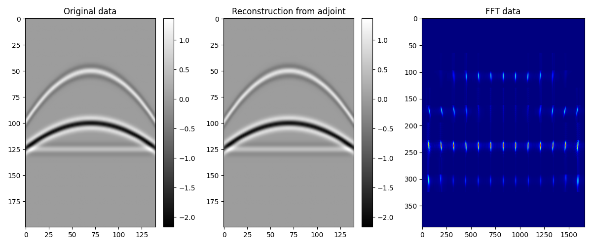
We want to divide this 2-dimensional data into small overlapping patches in the spatial direction and apply the adjoint of the pylops.signalprocessing.FFT2D operator to each patch. This is done by simply using the adjoint of the pylops.signalprocessing.Patch2D operator. Note that for non- orthogonal operators, this must be replaced by an inverse.

nwin = (20, 34)  # window size in data domain
nop = (
    128,
    128 // 2 + 1,
)  # window size in model domain; we use real FFT, second axis is half
nover = (10, 4)  # overlap between windows
dimsd = data.shape

# Sliding window transform without taper
Op = pylops.signalprocessing.FFT2D(nwin, nffts=(128, 128), real=True)

nwins, dims, mwin_inends, dwin_inends = pylops.signalprocessing.patch2d_design(
    dimsd, nwin, nover, (128, 65)
)
Patch = pylops.signalprocessing.Patch2D(
    Op.H, dims, dimsd, nwin, nover, nop, tapertype=None
)
fftdata = Patch.H * data

We now create a similar operator but we also add a taper to the overlapping parts of the patches. We then apply the forward to restore the original signal.

Patch = pylops.signalprocessing.Patch2D(
    Op.H, dims, dimsd, nwin, nover, nop, tapertype="hanning"
)

reconstructed_data = Patch * fftdata

Finally we re-arrange the transformed patches so that we can also display them

fftdatareshaped = np.zeros((nop[0] * nwins[0], nop[1] * nwins[1]), dtype=fftdata.dtype)

iwin = 1
for ix in range(nwins[0]):
    for it in range(nwins[1]):
        fftdatareshaped[
            ix * nop[0] : (ix + 1) * nop[0], it * nop[1] : (it + 1) * nop[1]
        ] = np.fft.fftshift(fftdata[ix, it])
        iwin += 1

Let’s finally visualize all the intermediate results as well as our final data reconstruction after inverting the pylops.signalprocessing.Sliding2D operator.

fig, axs = plt.subplots(1, 3, figsize=(12, 5))
im = axs[0].imshow(data.T, cmap="gray")
axs[0].set_title("Original data")
plt.colorbar(im, ax=axs[0])
axs[0].axis("tight")
im = axs[1].imshow(reconstructed_data.real.T, cmap="gray")
axs[1].set_title("Reconstruction from adjoint")
plt.colorbar(im, ax=axs[1])
axs[1].axis("tight")
axs[2].imshow(np.abs(fftdatareshaped).T, cmap="jet")
axs[2].set_title("FFT data")
axs[2].axis("tight")
plt.tight_layout()

We repeat now the same exercise in 3d

par = {
    "oy": -60,
    "dy": 2,
    "ny": 60,
    "ox": -50,
    "dx": 2,
    "nx": 50,
    "ot": 0,
    "dt": 0.004,
    "nt": 100,
    "f0": 20,
}

v = 1500
t0 = [0.05, 0.2, 0.3]
vrms = [500, 700, 1700]
amp = [1.0, -2, 0.5]

# Create axis
t, t2, x, y = pylops.utils.seismicevents.makeaxis(par)

# Create wavelet
wav = pylops.utils.wavelets.ricker(t[:41], f0=par["f0"])[0]

# Generate model
_, data = pylops.utils.seismicevents.hyperbolic3d(x, y, t, t0, vrms, vrms, amp, wav)


fig, axs = plt.subplots(1, 3, figsize=(12, 5))
fig.suptitle("Original data", fontsize=12, fontweight="bold", y=0.95)
axs[0].imshow(
    data[par["ny"] // 2].T,
    aspect="auto",
    interpolation="nearest",
    vmin=-2,
    vmax=2,
    cmap="gray",
    extent=(x.min(), x.max(), t.max(), t.min()),
)
axs[0].set_xlabel(r"$x(m)$")
axs[0].set_ylabel(r"$t(s)$")
axs[1].imshow(
    data[:, par["nx"] // 2].T,
    aspect="auto",
    interpolation="nearest",
    vmin=-2,
    vmax=2,
    cmap="gray",
    extent=(y.min(), y.max(), t.max(), t.min()),
)
axs[1].set_xlabel(r"$y(m)$")
axs[1].set_ylabel(r"$t(s)$")
axs[2].imshow(
    data[:, :, par["nt"] // 2],
    aspect="auto",
    interpolation="nearest",
    vmin=-2,
    vmax=2,
    cmap="gray",
    extent=(x.min(), x.max(), y.max(), x.min()),
)
axs[2].set_xlabel(r"$x(m)$")
axs[2].set_ylabel(r"$y(m)$")
plt.tight_layout()

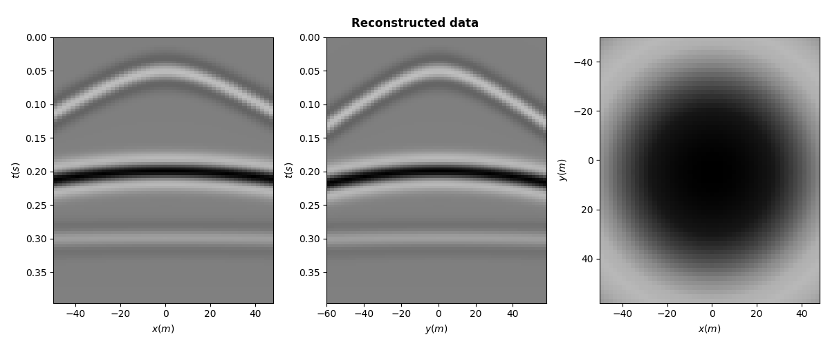
Let’s create now the pylops.signalprocessing.Patch3D operator applying the adjoint of the pylops.signalprocessing.FFT3D operator to each patch.

nwin = (20, 20, 34)  # window size in data domain
nop = (
    128,
    128,
    128 // 2 + 1,
)  # window size in model domain; we use real FFT, third axis is half
nover = (10, 10, 4)  # overlap between windows
dimsd = data.shape

# Sliding window transform without taper
Op = pylops.signalprocessing.FFTND(nwin, nffts=(128, 128, 128), real=True)

nwins, dims, mwin_inends, dwin_inends = pylops.signalprocessing.patch3d_design(
    dimsd, nwin, nover, (128, 128, 65)
)
Patch = pylops.signalprocessing.Patch3D(
    Op.H, dims, dimsd, nwin, nover, nop, tapertype=None
)
fftdata = Patch.H * data

Patch = pylops.signalprocessing.Patch3D(
    Op.H, dims, dimsd, nwin, nover, nop, tapertype="hanning"
)
reconstructed_data = np.real(Patch * fftdata)

fig, axs = plt.subplots(1, 3, figsize=(12, 5))
fig.suptitle("Reconstructed data", fontsize=12, fontweight="bold", y=0.95)
axs[0].imshow(
    reconstructed_data[par["ny"] // 2].T,
    aspect="auto",
    interpolation="nearest",
    vmin=-2,
    vmax=2,
    cmap="gray",
    extent=(x.min(), x.max(), t.max(), t.min()),
)
axs[0].set_xlabel(r"$x(m)$")
axs[0].set_ylabel(r"$t(s)$")
axs[1].imshow(
    reconstructed_data[:, par["nx"] // 2].T,
    aspect="auto",
    interpolation="nearest",
    vmin=-2,
    vmax=2,
    cmap="gray",
    extent=(y.min(), y.max(), t.max(), t.min()),
)
axs[1].set_xlabel(r"$y(m)$")
axs[1].set_ylabel(r"$t(s)$")
axs[2].imshow(
    reconstructed_data[:, :, par["nt"] // 2],
    aspect="auto",
    interpolation="nearest",
    vmin=-2,
    vmax=2,
    cmap="gray",
    extent=(x.min(), x.max(), y.max(), x.min()),
)
axs[2].set_xlabel(r"$x(m)$")
axs[2].set_ylabel(r"$y(m)$")
plt.tight_layout()