Note
Go to the end to download the full example code.
16. CT Scan Imaging
This tutorial considers a very well-known inverse problem from the field of medical imaging.
First, we will be using the pylops.signalprocessing.Radon2D operator
to model a sinogram, which is a graphic representation of the raw data
obtained from a CT scan.
Note that whilst we can twick the Radon2D operator to work in a CT-like style,
this has initially been designed with other applications in mind
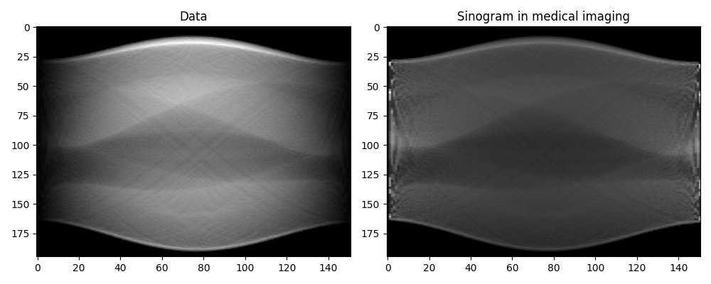
(i.e., seismic). We will see that if we use pylops.medical.CT2D the produced
sinogram will be very similar in the middle (horizontal and near horizontal lines) but
it will greatly differ at both end (vertical and near vertical lines). The latter lines
are in fact not easy to parametrize using the convention chosen in Radon2D.
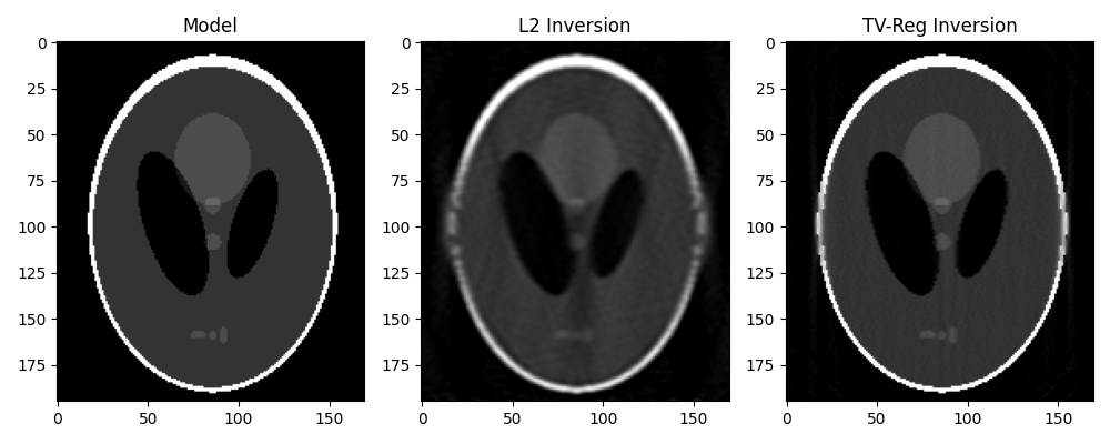
The sinogram created by the pylops.medical.CT2D operator is further
inverted using both a L2 solver and a TV-regularized solver like Split-Bregman.
import matplotlib.pyplot as plt

# sphinx_gallery_thumbnail_number = 2
import numpy as np
from numba import jit

import pylops

plt.close("all")
np.random.seed(10)
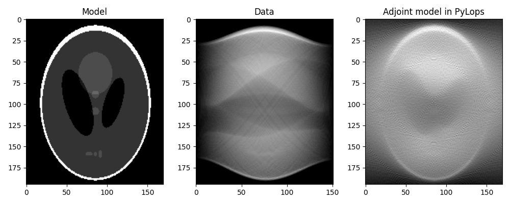
Let’s start by loading the Shepp-Logan phantom model. We can then construct
the sinogram by providing a custom-made function to the
pylops.signalprocessing.Radon2D that samples parametric curves of
such a type:
where \(\theta\) is the angle between the x-axis (\(x\)) and the perpendicular to the summation line and \(r\) is the distance from the origin of the summation line.
@jit(nopython=True)
def radoncurve(x, r, theta):
    return (
        (r - ny // 2) / (np.sin(theta) + 1e-15)
        + np.tan(np.pi / 2.0 - theta) * x
        + ny // 2
    )


x = np.load("../testdata/optimization/shepp_logan_phantom.npy").T
x = x / x.max()
nx, ny = x.shape

ntheta = 151
theta = np.linspace(0.0, np.pi, ntheta, endpoint=False)

RLop = pylops.signalprocessing.Radon2D(
    np.arange(ny),
    np.arange(nx),
    theta,
    kind=radoncurve,
    centeredh=True,
    interp=False,
    engine="numba",
    dtype="float64",
)

y = RLop.H * x
We can now first perform the adjoint, which in the medical imaging literature is also referred to as back-projection.
This is the first step of a common reconstruction technique, named filtered back-projection, which simply applies a correction filter in the frequency domain to the adjoint model.
xrec = RLop * y

fig, axs = plt.subplots(1, 3, figsize=(10, 4))
axs[0].imshow(x.T, vmin=0, vmax=1, cmap="gray")
axs[0].set_title("Model")
axs[0].axis("tight")
axs[1].imshow(y.T, cmap="gray")
axs[1].set_title("Data")
axs[1].axis("tight")
axs[2].imshow(xrec.T, cmap="gray")
axs[2].set_title("Adjoint model")
axs[2].axis("tight")
fig.tight_layout()
Let’s now repeat the same exercise, this time using the CT2D operator
Cop = pylops.medical.CT2D((ny, nx), 1.0, ny, theta, engine='cpu')

y = Cop * x.T
xrec = Cop.H * y

fig, axs = plt.subplots(1, 3, figsize=(10, 4))
axs[0].imshow(x.T, vmin=0, vmax=1, cmap="gray")
axs[0].set_title("Model")
axs[0].axis("tight")
axs[1].imshow(np.flipud(y.T), cmap="gray")
axs[1].set_title("Data")
axs[1].axis("tight")
axs[2].imshow(xrec, cmap="gray")
axs[2].set_title("Adjoint model")
axs[2].axis("tight")
fig.tight_layout()
Finally we take advantage of our different solvers and try to invert the modelling operator both in a least-squares sense and using TV-reg.
Dop = [
    pylops.FirstDerivative(
        (ny, nx), axis=0, edge=True, kind="backward", dtype=np.float64
    ),
    pylops.FirstDerivative(
        (ny, nx), axis=1, edge=True, kind="backward", dtype=np.float64
    ),
]
D2op = pylops.Laplacian(dims=(ny, nx), edge=True, dtype=np.float64)

# L2
xinv_sm = pylops.optimization.leastsquares.regularized_inversion(
    Cop, y.ravel(), [D2op], epsRs=[1e1], **dict(iter_lim=20)
)[0]
xinv_sm = np.real(xinv_sm.reshape(ny, nx)).T

# TV
mu = 1.5
lamda = [1.0, 1.0]
niter = 3
niterinner = 4

xinv = pylops.optimization.sparsity.splitbregman(
    Cop,
    y.ravel(),
    Dop,
    niter_outer=niter,
    niter_inner=niterinner,
    mu=mu,
    epsRL1s=lamda,
    tol=1e-4,
    tau=1.0,
    show=False,
    **dict(iter_lim=20, damp=1e-2)
)[0]
xinv = np.real(xinv.reshape(ny, nx)).T

fig, axs = plt.subplots(1, 3, figsize=(10, 4))
axs[0].imshow(x.T, vmin=0, vmax=1, cmap="gray")
axs[0].set_title("Model")
axs[0].axis("tight")
axs[1].imshow(xinv_sm.T, vmin=0, vmax=1, cmap="gray")
axs[1].set_title("L2 Inversion")
axs[1].axis("tight")
axs[2].imshow(xinv.T, vmin=0, vmax=1, cmap="gray")
axs[2].set_title("TV-Reg Inversion")
axs[2].axis("tight")
fig.tight_layout()
Total running time of the script: (0 minutes 44.300 seconds)