Fourier Transform

This example shows how to use the pylops.signalprocessing.FFT, pylops.signalprocessing.FFT2D and pylops.signalprocessing.FFTND operators to apply the Fourier Transform to the model and the inverse Fourier Transform to the data.

import matplotlib.pyplot as plt
import numpy as np

import pylops

plt.close("all")

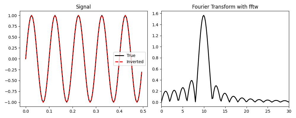
Let’s start by applying the one dimensional FFT to a one dimensional sinusoidal signal \(d(t)=sin(2 \pi f_0t)\) using a time axis of lenght \(nt\) and sampling \(dt\)

dt = 0.005
nt = 100
t = np.arange(nt) * dt
f0 = 10
nfft = 2**10
d = np.sin(2 * np.pi * f0 * t)

FFTop = pylops.signalprocessing.FFT(dims=nt, nfft=nfft, sampling=dt, engine="numpy")
D = FFTop * d

# Adjoint = inverse for FFT
dinv = FFTop.H * D
dinv = FFTop / D

fig, axs = plt.subplots(1, 2, figsize=(10, 4))
axs[0].plot(t, d, "k", lw=2, label="True")
axs[0].plot(t, dinv.real, "--r", lw=2, label="Inverted")
axs[0].legend()
axs[0].set_title("Signal")
axs[1].plot(FFTop.f[: int(FFTop.nfft / 2)], np.abs(D[: int(FFTop.nfft / 2)]), "k", lw=2)
axs[1].set_title("Fourier Transform")
axs[1].set_xlim([0, 3 * f0])
plt.tight_layout()

In this example we used numpy as our engine for the fft and ifft. PyLops implements a second engine (engine='fftw') which uses the well-known FFTW via the python wrapper pyfftw.FFTW. This optimized fft tends to outperform the one from numpy in many cases but it is not inserted in the mandatory requirements of PyLops. If interested to use FFTW backend, read the fft routines section at Advanced installation.

FFTop = pylops.signalprocessing.FFT(dims=nt, nfft=nfft, sampling=dt, engine="fftw")
D = FFTop * d

# Adjoint = inverse for FFT
dinv = FFTop.H * D
dinv = FFTop / D

fig, axs = plt.subplots(1, 2, figsize=(10, 4))
axs[0].plot(t, d, "k", lw=2, label="True")
axs[0].plot(t, dinv.real, "--r", lw=2, label="Inverted")
axs[0].legend()
axs[0].set_title("Signal")
axs[1].plot(FFTop.f[: int(FFTop.nfft / 2)], np.abs(D[: int(FFTop.nfft / 2)]), "k", lw=2)
axs[1].set_title("Fourier Transform with fftw")
axs[1].set_xlim([0, 3 * f0])
plt.tight_layout()

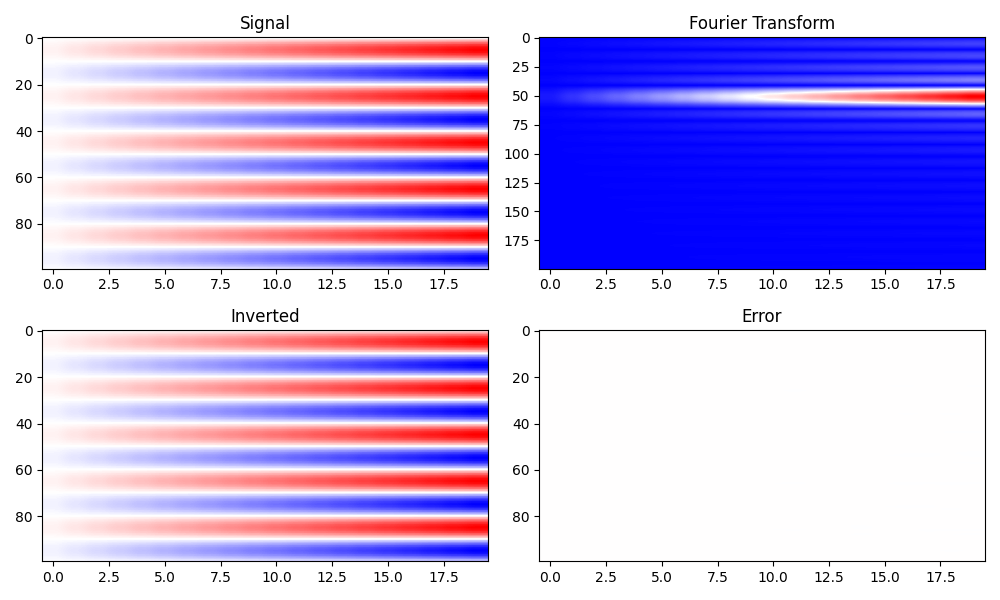
We can also apply the one dimensional FFT to to a two-dimensional signal (along one of the first axis)

dt = 0.005
nt, nx = 100, 20
t = np.arange(nt) * dt
f0 = 10
nfft = 2**10
d = np.outer(np.sin(2 * np.pi * f0 * t), np.arange(nx) + 1)

FFTop = pylops.signalprocessing.FFT(dims=(nt, nx), axis=0, nfft=nfft, sampling=dt)
D = FFTop * d.ravel()

# Adjoint = inverse for FFT
dinv = FFTop.H * D
dinv = FFTop / D
dinv = np.real(dinv).reshape(nt, nx)

fig, axs = plt.subplots(2, 2, figsize=(10, 6))
axs[0][0].imshow(d, vmin=-20, vmax=20, cmap="bwr")
axs[0][0].set_title("Signal")
axs[0][0].axis("tight")
axs[0][1].imshow(np.abs(D.reshape(nfft, nx)[:200, :]), cmap="bwr")
axs[0][1].set_title("Fourier Transform")
axs[0][1].axis("tight")
axs[1][0].imshow(dinv, vmin=-20, vmax=20, cmap="bwr")
axs[1][0].set_title("Inverted")
axs[1][0].axis("tight")
axs[1][1].imshow(d - dinv, vmin=-20, vmax=20, cmap="bwr")
axs[1][1].set_title("Error")
axs[1][1].axis("tight")
fig.tight_layout()

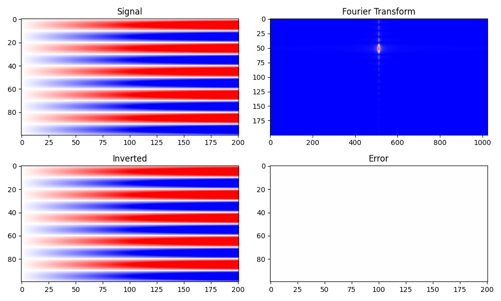
We can also apply the two dimensional FFT to to a two-dimensional signal

dt, dx = 0.005, 5
nt, nx = 100, 201
t = np.arange(nt) * dt
x = np.arange(nx) * dx
f0 = 10
nfft = 2**10
d = np.outer(np.sin(2 * np.pi * f0 * t), np.arange(nx) + 1)

FFTop = pylops.signalprocessing.FFT2D(
    dims=(nt, nx), nffts=(nfft, nfft), sampling=(dt, dx)
)
D = FFTop * d.ravel()

dinv = FFTop.H * D
dinv = FFTop / D
dinv = np.real(dinv).reshape(nt, nx)

fig, axs = plt.subplots(2, 2, figsize=(10, 6))
axs[0][0].imshow(d, vmin=-100, vmax=100, cmap="bwr")
axs[0][0].set_title("Signal")
axs[0][0].axis("tight")
axs[0][1].imshow(
    np.abs(np.fft.fftshift(D.reshape(nfft, nfft), axes=1)[:200, :]), cmap="bwr"
)
axs[0][1].set_title("Fourier Transform")
axs[0][1].axis("tight")
axs[1][0].imshow(dinv, vmin=-100, vmax=100, cmap="bwr")
axs[1][0].set_title("Inverted")
axs[1][0].axis("tight")
axs[1][1].imshow(d - dinv, vmin=-100, vmax=100, cmap="bwr")
axs[1][1].set_title("Error")
axs[1][1].axis("tight")
fig.tight_layout()

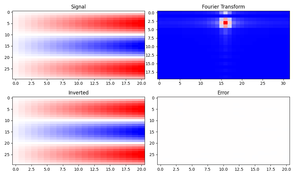
Finally can apply the three dimensional FFT to to a three-dimensional signal

dt, dx, dy = 0.005, 5, 3
nt, nx, ny = 30, 21, 11
t = np.arange(nt) * dt
x = np.arange(nx) * dx
y = np.arange(nx) * dy
f0 = 10
nfft = 2**6
nfftk = 2**5

d = np.outer(np.sin(2 * np.pi * f0 * t), np.arange(nx) + 1)
d = np.tile(d[:, :, np.newaxis], [1, 1, ny])

FFTop = pylops.signalprocessing.FFTND(
    dims=(nt, nx, ny), nffts=(nfft, nfftk, nfftk), sampling=(dt, dx, dy)
)
D = FFTop * d.ravel()

dinv = FFTop.H * D
dinv = FFTop / D
dinv = np.real(dinv).reshape(nt, nx, ny)

fig, axs = plt.subplots(2, 2, figsize=(10, 6))
axs[0][0].imshow(d[:, :, ny // 2], vmin=-20, vmax=20, cmap="bwr")
axs[0][0].set_title("Signal")
axs[0][0].axis("tight")
axs[0][1].imshow(
    np.abs(np.fft.fftshift(D.reshape(nfft, nfftk, nfftk), axes=1)[:20, :, nfftk // 2]),
    cmap="bwr",
)
axs[0][1].set_title("Fourier Transform")
axs[0][1].axis("tight")
axs[1][0].imshow(dinv[:, :, ny // 2], vmin=-20, vmax=20, cmap="bwr")
axs[1][0].set_title("Inverted")
axs[1][0].axis("tight")
axs[1][1].imshow(d[:, :, ny // 2] - dinv[:, :, ny // 2], vmin=-20, vmax=20, cmap="bwr")
axs[1][1].set_title("Error")
axs[1][1].axis("tight")
fig.tight_layout()