pylops.signalprocessing.NonStationaryConvolve1D#
- class pylops.signalprocessing.NonStationaryConvolve1D(dims, hs, ih, axis=-1, dtype='float64', name='C')[source]#
1D non-stationary convolution operator.
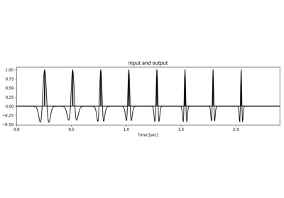
Apply non-stationary one-dimensional convolution. A varying compact filter is provided on a coarser grid and on-the-fly interpolation is applied in forward and adjoint modes.
- Parameters
- dims
listorint Number of samples for each dimension
- hs
numpy.ndarray Bank of 1d compact filters of size \(n_\text{filts} \times n_h\). Filters must have odd number of samples and are assumed to be centered in the middle of the filter support.
- ih
tuple Indices of the locations of the filters
hsin the model (and data). Note that the filters must be regularly sampled, i.e. \(dh=\text{diff}(ih)=\text{const.}\)- axis
int, optional Axis along which convolution is applied
- dtype
str, optional Type of elements in input array.
- name
str, optional Name of operator (to be used by
pylops.utils.describe.describe)
- dims
- Raises
- ValueError
If filters
hshave even size- ValueError
If
ihis not regularly sampled- ValueError
If
ihis outside the bounds defined bydims[axis]
Notes
The NonStationaryConvolve1D operator applies non-stationary one-dimensional convolution between the input signal \(d(t)\) and a bank of compact filter kernels \(h(t; t_i)\). Assuming an input signal composed of \(N=5\) samples, and filters at locations \(t_1\) and \(t_3\), the forward operator can be represented as follows:
\[\begin{split}\mathbf{y} = \begin{bmatrix} \hat{h}_{0,0} & h_{1,0} & \hat{h}_{2,0} & h_{3,0} & \hat{h}_{4,0} \\ \hat{h}_{0,1} & h_{1,1} & \hat{h}_{2,1} & h_{3,1} & \hat{h}_{4,1} \\ \vdots & \vdots & \vdots & \vdots & \vdots \\ \hat{h}_{0,4} & h_{1,4} & \hat{h}_{2,4} & h_{3,4} & \hat{h}_{4,4} \\ \end{bmatrix} \begin{bmatrix} x_0 \\ x_1 \\ \vdots \\ x_4 \end{bmatrix}\end{split}\]where \(\mathbf{h}_1 = [h_{1,0}, h_{1,1}, \ldots, h_{1,N}]\) and \(\mathbf{h}_3 = [h_{3,0}, h_{3,1}, \ldots, h_{3,N}]\) are the provided filter, \(\hat{\mathbf{h}}_0 = \mathbf{h}_1\) and \(\hat{\mathbf{h}}_4 = \mathbf{h}_3\) are the filters outside the range of the provided filters (which are extrapolated to be the same as the nearest provided filter) and \(\hat{\mathbf{h}}_2 = 0.5 \mathbf{h}_1 + 0.5 \mathbf{h}_3\) is the filter within the range of the provided filters (which is linearly interpolated from the two nearest provided filter on either side of its location).
In forward mode, each filter is weighted by the corresponding input and spread over the output. In adjoint mode, the corresponding filter is element-wise multiplied with the input, all values are summed together and put in the output.
- Attributes
- shape
tuple Operator shape
- explicit
bool Operator contains a matrix that can be solved explicitly (
True) or not (False)
- shape
Methods
__init__(dims, hs, ih[, axis, dtype, name])adjoint()apply_columns(cols)Apply subset of columns of operator
cond([uselobpcg])Condition number of linear operator.
conj()Complex conjugate operator
div(y[, niter, densesolver])Solve the linear problem \(\mathbf{y}=\mathbf{A}\mathbf{x}\).
dot(x)Matrix-matrix or matrix-vector multiplication.
eigs([neigs, symmetric, niter, uselobpcg])Most significant eigenvalues of linear operator.
matmat(X)Matrix-matrix multiplication.
matvec(x)Matrix-vector multiplication.
reset_count()Reset counters
rmatmat(X)Matrix-matrix multiplication.
rmatvec(x)Adjoint matrix-vector multiplication.
todense()Return dense matrix.
toimag([forw, adj])Imag operator
toreal([forw, adj])Real operator
tosparse()Return sparse matrix.
trace([neval, method, backend])Trace of linear operator.
transpose()
