Note
Go to the end to download the full example code.
Matrix Multiplication
This example shows how to use the pylops.MatrixMult operator
to perform Matrix inversion of the following linear system.
You will see that since this operator is a simple overloading to a
numpy.ndarray object, the solution of the linear system
can be obtained via both direct inversion (i.e., by means explicit
solver such as scipy.linalg.solve or scipy.linalg.lstsq)
and iterative solver (i.e., from scipy.sparse.linalg.lsqr).
Note that in case of rectangular \(\mathbf{A}\), an exact inverse does not exist and a least-square solution is computed instead.
import warnings

import matplotlib.gridspec as pltgs
import matplotlib.pyplot as plt
import numpy as np
from scipy.sparse import rand
from scipy.sparse.linalg import lsqr

import pylops

plt.close("all")
warnings.filterwarnings("ignore")
# sphinx_gallery_thumbnail_number = 2
Let’s define the sizes of the matrix \(\mathbf{A}\) (N and M) and
fill the matrix with random numbers
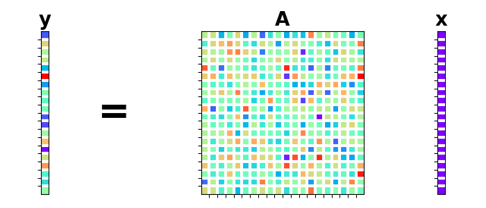
We can now apply the forward operator to create the data vector \(\mathbf{y}\)
and use / to solve the system by means of an explicit solver.
Let’s visually plot the system of equations we just solved.
gs = pltgs.GridSpec(1, 6)
fig = plt.figure(figsize=(7, 3))
ax = plt.subplot(gs[0, 0])
ax.imshow(y[:, np.newaxis], cmap="rainbow")
ax.set_title("y", size=20, fontweight="bold")
ax.set_xticks([])
ax.set_yticks(np.arange(N - 1) + 0.5)
ax.grid(linewidth=3, color="white")
ax.xaxis.set_ticklabels([])
ax.yaxis.set_ticklabels([])
ax = plt.subplot(gs[0, 1])
ax.text(
0.35,
0.5,
"=",
horizontalalignment="center",
verticalalignment="center",
size=40,
fontweight="bold",
)
ax.axis("off")
ax = plt.subplot(gs[0, 2:5])
ax.imshow(Aop.A, cmap="rainbow")
ax.set_title("A", size=20, fontweight="bold")
ax.set_xticks(np.arange(N - 1) + 0.5)
ax.set_yticks(np.arange(M - 1) + 0.5)
ax.grid(linewidth=3, color="white")
ax.xaxis.set_ticklabels([])
ax.yaxis.set_ticklabels([])
ax = plt.subplot(gs[0, 5])
ax.imshow(x[:, np.newaxis], cmap="rainbow")
ax.set_title("x", size=20, fontweight="bold")
ax.set_xticks([])
ax.set_yticks(np.arange(M - 1) + 0.5)
ax.grid(linewidth=3, color="white")
ax.xaxis.set_ticklabels([])
ax.yaxis.set_ticklabels([])
plt.tight_layout()
gs = pltgs.GridSpec(1, 6)
fig = plt.figure(figsize=(7, 3))
ax = plt.subplot(gs[0, 0])
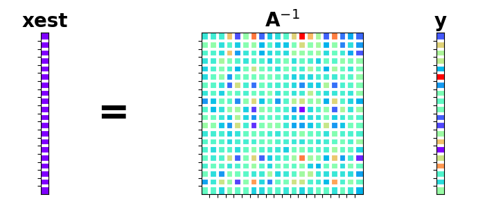
ax.imshow(x[:, np.newaxis], cmap="rainbow")
ax.set_title("xest", size=20, fontweight="bold")
ax.set_xticks([])
ax.set_yticks(np.arange(M - 1) + 0.5)
ax.grid(linewidth=3, color="white")
ax.xaxis.set_ticklabels([])
ax.yaxis.set_ticklabels([])
ax = plt.subplot(gs[0, 1])
ax.text(
0.35,
0.5,
"=",
horizontalalignment="center",
verticalalignment="center",
size=40,
fontweight="bold",
)
ax.axis("off")
ax = plt.subplot(gs[0, 2:5])
ax.imshow(Aop.inv(), cmap="rainbow")
ax.set_title(r"A$^{-1}$", size=20, fontweight="bold")
ax.set_xticks(np.arange(N - 1) + 0.5)
ax.set_yticks(np.arange(M - 1) + 0.5)
ax.grid(linewidth=3, color="white")
ax.xaxis.set_ticklabels([])
ax.yaxis.set_ticklabels([])
ax = plt.subplot(gs[0, 5])
ax.imshow(y[:, np.newaxis], cmap="rainbow")
ax.set_title("y", size=20, fontweight="bold")
ax.set_xticks([])
ax.set_yticks(np.arange(N - 1) + 0.5)
ax.grid(linewidth=3, color="white")
ax.xaxis.set_ticklabels([])
ax.yaxis.set_ticklabels([])
plt.tight_layout()
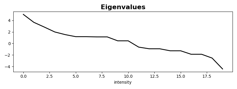
Let’s also plot the matrix eigenvalues
plt.figure(figsize=(8, 3))
plt.plot(Aop.eigs(), "k", lw=2)
plt.title("Eigenvalues", size=16, fontweight="bold")
plt.xlabel("#eigenvalue")
plt.xlabel("intensity")
plt.tight_layout()
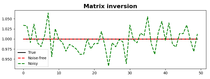
We can also repeat the same exercise for a non-square matrix
N, M = 200, 50
A = np.random.normal(0, 1, (N, M))
x = np.ones(M)

Aop = pylops.MatrixMult(A, dtype="float64")
y = Aop * x
yn = y + np.random.normal(0, 0.3, N)

xest = Aop / y
xnest = Aop / yn

plt.figure(figsize=(8, 3))
plt.plot(x, "k", lw=2, label="True")
plt.plot(xest, "--r", lw=2, label="Noise-free")
plt.plot(xnest, "--g", lw=2, label="Noisy")
plt.title("Matrix inversion", size=16, fontweight="bold")
plt.legend()
plt.tight_layout()
And we can also use a sparse matrix from the scipy.sparse
family of sparse matrices.
A= [[0.48401674 0.         0.72121322 0.64936939 0.72756114]
 [0.         0.90929906 0.33655684 0.32406567 0.68186319]
 [0.24919265 0.         0.4268735  0.04539436 0.42484727]
 [0.96149046 0.55511469 0.17580924 0.93124229 0.        ]
 [0.56324398 0.         0.         0.8321156  0.98046467]]
A^-1= [[-1.72658497 -0.55868992  2.98068176  0.91515541  0.37819996]
 [-0.73831115  0.85697344  0.40795381  0.39767433 -0.22488337]
 [ 1.45858004  0.04865949 -0.12722932 -0.0797061  -1.0610604 ]
 [ 1.94740993  0.05680765 -3.29666098 -0.09305311 -0.05611361]
 [-0.66089233  0.27273619  1.08555871 -0.44675229  0.85028475]]
eigs= [2.31216696+0.j         0.79482532+0.j         0.44488287-0.53315612j]
x= [1. 1. 1. 1. 1.]
y= [2.58216049 2.25178475 1.14630777 2.62365668 2.37582426]
lsqr solution xest= [1. 1. 1. 1. 1.]
Finally, in several circumstances the input model \(\mathbf{x}\) may be more naturally arranged as a matrix or a multi-dimensional array and it may be desirable to apply the same matrix to every columns of the model. This can be mathematically expressed as:
\[\begin{split}\mathbf{y} = \begin{bmatrix} \mathbf{A} \quad \mathbf{0} \quad \mathbf{0} \\ \mathbf{0} \quad \mathbf{A} \quad \mathbf{0} \\ \mathbf{0} \quad \mathbf{0} \quad \mathbf{A} \end{bmatrix} \begin{bmatrix} \mathbf{x_1} \\ \mathbf{x_2} \\ \mathbf{x_3} \end{bmatrix}\end{split}\]
and apply it using the same implementation of the
pylops.MatrixMult operator by simply telling the operator how we
want the model to be organized through the otherdims input parameter.
A = np.array([[1.0, 2.0], [4.0, 5.0]])
x = np.array([[1.0, 1.0], [2.0, 2.0], [3.0, 3.0]])

Aop = pylops.MatrixMult(A, otherdims=(3,), dtype="float64")
y = Aop * x.ravel()

xest, istop, itn, r1norm, r2norm = lsqr(Aop, y, damp=1e-10, iter_lim=10, show=0)[0:5]
xest = xest.reshape(3, 2)

print(f"A= {A}")
print(f"x= {x}")
print(f"y={y}")
print(f"lsqr solution xest= {xest}")
A= [[1. 2.]
 [4. 5.]]
x= [[1. 1.]
 [2. 2.]
 [3. 3.]]
y=[ 5.  7.  8. 14. 19. 23.]
lsqr solution xest= [[1. 1.]
 [2. 2.]
 [3. 3.]]
Total running time of the script: (0 minutes 0.691 seconds)