Note
Go to the end to download the full example code.
11. Radon filtering
In this example we will be taking advantage of the
pylops.signalprocessing.Radon2D operator to perform filtering of
unwanted events from a seismic data. For those of you not familiar with seismic
data, let’s imagine that we have a data composed of a certain number of flat
events and a parabolic event , we are after a transform that allows us to
separate such an event from the others and filter it out.
Those of you with a geophysics background may immediately realize this
is the case of seismic angle (or offset) gathers after migration and those
events with parabolic moveout are generally residual multiples that we would
like to suppress prior to performing further analysis of our data.
The Radon transform is actually a very good transform to perform such a separation. We can thus devise a simple workflow that takes our data as input, applies a Radon transform, filters some of the events out and goes back to the original domain.
import matplotlib.pyplot as plt
import numpy as np

import pylops
from pylops.utils.wavelets import ricker

plt.close("all")
np.random.seed(0)
Let’s first create a data composed on 3 linear events and a parabolic event.
par = {"ox": 0, "dx": 2, "nx": 121, "ot": 0, "dt": 0.004, "nt": 100, "f0": 30}

# linear events
v = 1500  # m/s
t0 = [0.1, 0.2, 0.3]  # s
theta = [0, 0, 0]
amp = [1.0, -2, 0.5]

# parabolic event
tp0 = [0.13]  # s
px = [0]  # s/m
pxx = [5e-7]  # s²/m²
ampp = [0.7]

# create axis
taxis, taxis2, xaxis, yaxis = pylops.utils.seismicevents.makeaxis(par)

# create wavelet
wav = ricker(taxis[:41], f0=par["f0"])[0]

# generate model
y = (
    pylops.utils.seismicevents.linear2d(xaxis, taxis, v, t0, theta, amp, wav)[1]
    + pylops.utils.seismicevents.parabolic2d(xaxis, taxis, tp0, px, pxx, ampp, wav)[1]
)
We can now create the pylops.signalprocessing.Radon2D operator.
We also apply its adjoint to the data to obtain a representation of those
3 linear events overlapping to a parabolic event in the Radon domain.
Similarly, we feed the operator to a sparse solver like
pylops.optimization.sparsity.FISTA to obtain a sparse
represention of the data in the Radon domain. At this point we try to filter
out the unwanted event. We can see how this is much easier for the sparse
transform as each event has a much more compact representation in the Radon
domain than for the adjoint transform.
# radon operator
npx = 61
pxmax = 5e-4  # s/m
px = np.linspace(-pxmax, pxmax, npx)

Rop = pylops.signalprocessing.Radon2D(
    taxis, xaxis, px, kind="linear", interp="nearest", centeredh=False, dtype="float64"
)

# adjoint Radon transform
xadj = Rop.H * y

# sparse Radon transform
xinv, niter, cost = pylops.optimization.sparsity.fista(
    Rop, y.ravel(), niter=15, eps=1e1
)
xinv = xinv.reshape(Rop.dims)

# filtering
xfilt = np.zeros_like(xadj)
xfilt[npx // 2 - 3 : npx // 2 + 4] = xadj[npx // 2 - 3 : npx // 2 + 4]

yfilt = Rop * xfilt

# filtering on sparse transform
xinvfilt = np.zeros_like(xinv)
xinvfilt[npx // 2 - 3 : npx // 2 + 4] = xinv[npx // 2 - 3 : npx // 2 + 4]

yinvfilt = Rop * xinvfilt
Finally we visualize our results.
pclip = 0.7
fig, axs = plt.subplots(1, 5, sharey=True, figsize=(12, 5))
axs[0].imshow(
    y.T,
    cmap="gray",
    vmin=-pclip * np.abs(y).max(),
    vmax=pclip * np.abs(y).max(),
    extent=(xaxis[0], xaxis[-1], taxis[-1], taxis[0]),
)
axs[0].set(xlabel="$x$ [m]", ylabel="$t$ [s]", title="Data")
axs[0].axis("tight")
axs[1].imshow(
    xadj.T,
    cmap="gray",
    vmin=-pclip * np.abs(xadj).max(),
    vmax=pclip * np.abs(xadj).max(),
    extent=(px[0], px[-1], taxis[-1], taxis[0]),
)
axs[1].axvline(px[npx // 2 - 3], color="r", linestyle="--")
axs[1].axvline(px[npx // 2 + 3], color="r", linestyle="--")
axs[1].set(xlabel="$p$ [s/m]", title="Radon")
axs[1].axis("tight")
axs[2].imshow(
    yfilt.T,
    cmap="gray",
    vmin=-pclip * np.abs(yfilt).max(),
    vmax=pclip * np.abs(yfilt).max(),
    extent=(xaxis[0], xaxis[-1], taxis[-1], taxis[0]),
)
axs[2].set(xlabel="$x$ [m]", title="Filtered data")
axs[2].axis("tight")
axs[3].imshow(
    xinv.T,
    cmap="gray",
    vmin=-pclip * np.abs(xinv).max(),
    vmax=pclip * np.abs(xinv).max(),
    extent=(px[0], px[-1], taxis[-1], taxis[0]),
)
axs[3].axvline(px[npx // 2 - 3], color="r", linestyle="--")
axs[3].axvline(px[npx // 2 + 3], color="r", linestyle="--")
axs[3].set(xlabel="$p$ [s/m]", title="Sparse Radon")
axs[3].axis("tight")
axs[4].imshow(
    yinvfilt.T,
    cmap="gray",
    vmin=-pclip * np.abs(y).max(),
    vmax=pclip * np.abs(y).max(),
    extent=(xaxis[0], xaxis[-1], taxis[-1], taxis[0]),
)

axs[4].set(xlabel="$x$ [m]", title="Sparse filtered data")
axs[4].axis("tight")
plt.tight_layout()
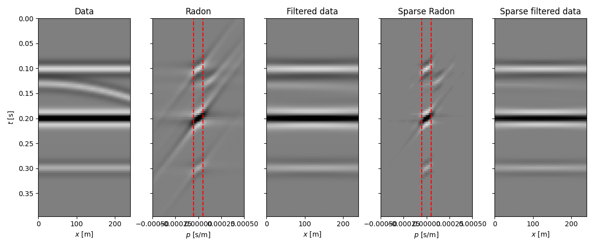
As expected, the Radon domain is a suitable domain for this type of filtering and the sparse transform improves the ability to filter out parabolic events with small curvature.
On the other hand, it is important to note that we have not been able to correctly preserve the amplitudes of each event. This is because the sparse Radon transform can only identify a sparsest response that explain the data within a certain threshold. For this reason a more suitable approach for preserving amplitudes could be to apply a parabolic Raodn transform with the aim of reconstructing only the unwanted event and apply an adaptive subtraction between the input data and the reconstructed unwanted event.
Total running time of the script: (0 minutes 15.988 seconds)