Seislet transform

This example shows how to use the pylops.signalprocessing.Seislet operator. This operator the forward, adjoint and inverse Seislet transform that is a modification of the well-know Wavelet transform where local slopes are used in the prediction and update steps to further improve the prediction of a trace from its previous (or subsequent) one and reduce the amount of information passed to the subsequent scale. While this transform was initially developed in the context of processing and compression of seismic data, it is also suitable to any other oscillatory dataset such as GPR or Acoustic recordings.

import matplotlib.pyplot as plt
import numpy as np
from matplotlib.ticker import MaxNLocator
from mpl_toolkits.axes_grid1 import make_axes_locatable

import pylops

plt.close("all")

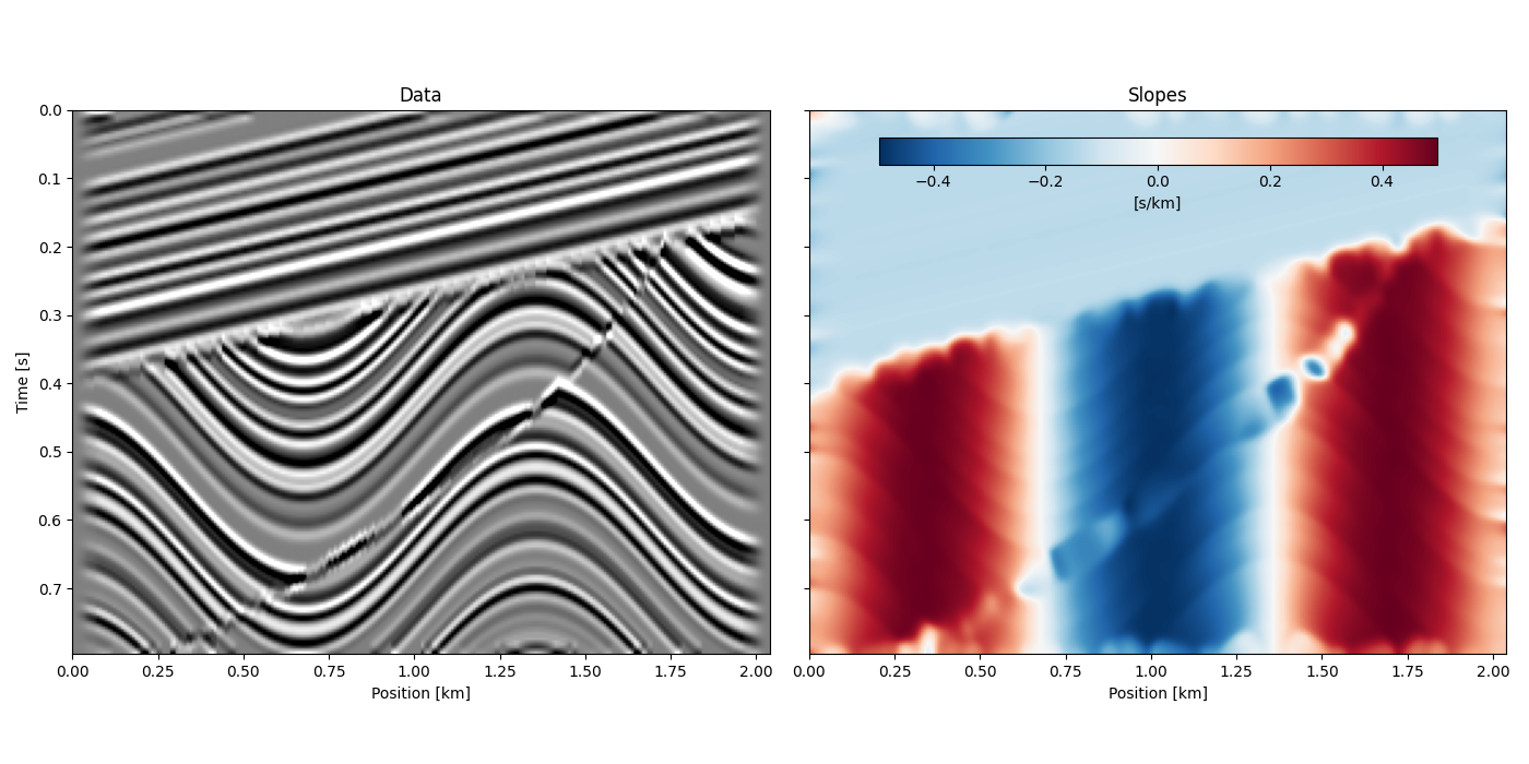
In this example we use the same benchmark dataset that was used in the original paper describing the Seislet transform. First, local slopes are estimated using pylops.utils.signalprocessing.slope_estimate.

inputfile = "../testdata/sigmoid.npz"

d = np.load(inputfile)
d = d["sigmoid"]
nx, nt = d.shape
dx, dt = 0.008, 0.004
x, t = np.arange(nx) * dx, np.arange(nt) * dt

# slope estimation
slope, _ = pylops.utils.signalprocessing.slope_estimate(d.T, dt, dx, smooth=2.5)
slope = -slope.T  # t-axis points down, reshape
# clip slopes above 80°
pmax = np.arctan(80 * np.pi / 180)
slope[slope > pmax] = pmax
slope[slope < -pmax] = -pmax

clip = 0.5 * np.max(np.abs(d))
clip_s = min(pmax, np.max(np.abs(slope)))
opts = dict(aspect=2, extent=(x[0], x[-1], t[-1], t[0]))

fig, axs = plt.subplots(1, 2, figsize=(14, 7), sharey=True, sharex=True)
axs[0].imshow(d.T, cmap="gray", vmin=-clip, vmax=clip, **opts)
axs[0].set(xlabel="Position [km]", ylabel="Time [s]", title="Data")

im = axs[1].imshow(slope.T, cmap="RdBu_r", vmin=-clip_s, vmax=clip_s, **opts)
axs[1].set(xlabel="Position [km]", title="Slopes")
fig.tight_layout()

pos = axs[1].get_position()
cbpos = [
    pos.x0 + 0.1 * pos.width,
    pos.y0 + 0.9 * pos.height,
    0.8 * pos.width,
    0.05 * pos.height,
]
cax = fig.add_axes(cbpos)
cb = fig.colorbar(im, cax=cax, orientation="horizontal")
cb.set_label("[s/km]")

Next the Seislet transform is computed.

Sop = pylops.signalprocessing.Seislet(slope, sampling=(dx, dt))

seis = Sop * d

nlevels_max = int(np.log2(nx))
levels_size = np.flip(np.array([2**i for i in range(nlevels_max)]))
levels_cum = np.cumsum(levels_size)

fig, ax = plt.subplots(figsize=(14, 6))
im = ax.imshow(
    seis.T,
    cmap="gray",
    vmin=-clip,
    vmax=clip,
    aspect="auto",
    interpolation="none",
    extent=(1, seis.shape[0], t[-1], t[0]),
)
ax.xaxis.set_major_locator(MaxNLocator(nbins=20, integer=True))
for level in levels_cum:
    ax.axvline(level + 0.5, color="w")
ax.set(xlabel="Scale", ylabel="Time [s]", title="Seislet transform")
cax = make_axes_locatable(ax).append_axes("right", size="2%", pad=0.1)
cb = fig.colorbar(im, cax=cax, orientation="vertical")
cb.formatter.set_powerlimits((0, 0))
fig.tight_layout()

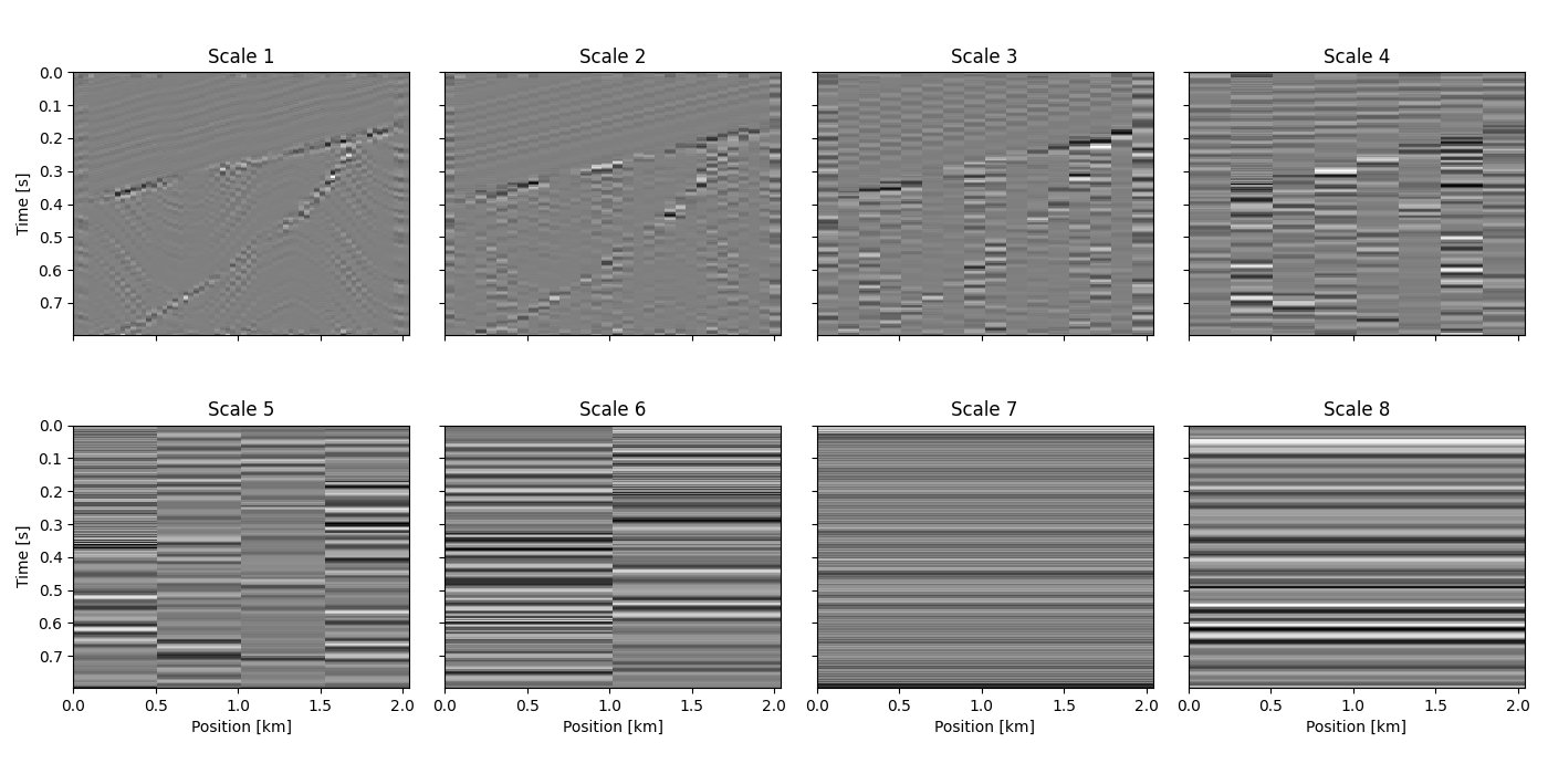
We may also stretch the finer scales to be the width of the image

fig, axs = plt.subplots(2, nlevels_max // 2, figsize=(14, 7), sharex=True, sharey=True)
for i, ax in enumerate(axs.ravel()[:-1]):
    curdata = seis[levels_cum[i] : levels_cum[i + 1], :].T
    vmax = np.max(np.abs(curdata))
    ax.imshow(curdata, vmin=-vmax, vmax=vmax, cmap="gray", interpolation="none", **opts)
    ax.set(title=f"Scale {i+1}")
    if i + 1 > nlevels_max // 2:
        ax.set(xlabel="Position [km]")
curdata = seis[levels_cum[-1] :, :].T
vmax = np.max(np.abs(curdata))
axs[-1, -1].imshow(
    curdata, vmin=-vmax, vmax=vmax, cmap="gray", interpolation="none", **opts
)
axs[0, 0].set(ylabel="Time [s]")
axs[1, 0].set(ylabel="Time [s]")
axs[-1, -1].set(xlabel="Position [km]", title=f"Scale {nlevels_max}")
fig.tight_layout()

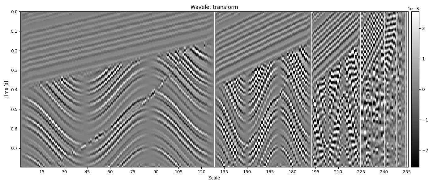
As a comparison we also compute the Seislet transform fixing slopes to zero. This way we turn the Seislet tranform into a basic 1D Wavelet transform performed over the spatial axis.

Wop = pylops.signalprocessing.Seislet(np.zeros_like(slope), sampling=(dx, dt))
dwt = Wop * d

fig, ax = plt.subplots(figsize=(14, 6))
im = ax.imshow(
    dwt.T,
    cmap="gray",
    vmin=-clip,
    vmax=clip,
    aspect="auto",
    interpolation="none",
    extent=(1, dwt.shape[0], t[-1], t[0]),
)
ax.xaxis.set_major_locator(MaxNLocator(nbins=20, integer=True))
for level in levels_cum:
    ax.axvline(level + 0.5, color="w")
ax.set(xlabel="Scale", ylabel="Time [s]", title="Wavelet transform")
cax = make_axes_locatable(ax).append_axes("right", size="2%", pad=0.1)
cb = fig.colorbar(im, cax=cax, orientation="vertical")
cb.formatter.set_powerlimits((0, 0))
fig.tight_layout()

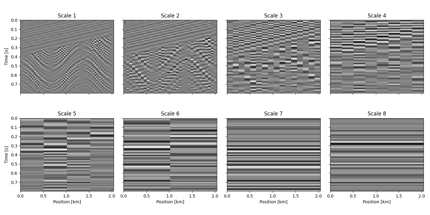
Again, we may decompress the finer scales

fig, axs = plt.subplots(2, nlevels_max // 2, figsize=(14, 7), sharex=True, sharey=True)
for i, ax in enumerate(axs.ravel()[:-1]):
    curdata = dwt[levels_cum[i] : levels_cum[i + 1], :].T
    vmax = np.max(np.abs(curdata))
    ax.imshow(curdata, vmin=-vmax, vmax=vmax, cmap="gray", interpolation="none", **opts)
    ax.set(title=f"Scale {i+1}")
    if i + 1 > nlevels_max // 2:
        ax.set(xlabel="Position [km]")
curdata = dwt[levels_cum[-1] :, :].T
vmax = np.max(np.abs(curdata))
axs[-1, -1].imshow(
    curdata, vmin=-vmax, vmax=vmax, cmap="gray", interpolation="none", **opts
)
axs[0, 0].set(ylabel="Time [s]")
axs[1, 0].set(ylabel="Time [s]")
axs[-1, -1].set(xlabel="Position [km]", title=f"Scale {nlevels_max}")
fig.tight_layout()

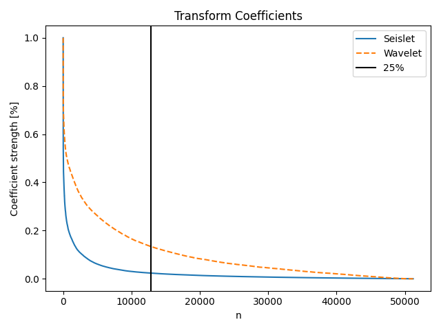
Finally we evaluate the compression capabilities of the Seislet transform compared to the 1D Wavelet transform. We zero-out all but the strongest 25% of the components. We perform the inverse transforms and assess the compression error.

perc = 0.25
seis_strong_idx = np.argsort(-np.abs(seis.ravel()))
dwt_strong_idx = np.argsort(-np.abs(dwt.ravel()))
seis_strong = np.abs(seis.ravel())[seis_strong_idx]
dwt_strong = np.abs(dwt.ravel())[dwt_strong_idx]

fig, ax = plt.subplots()
ax.plot(range(1, len(seis_strong) + 1), seis_strong / seis_strong[0], label="Seislet")
ax.plot(
    range(1, len(dwt_strong) + 1), dwt_strong / dwt_strong[0], "--", label="Wavelet"
)
ax.set(xlabel="n", ylabel="Coefficient strength [%]", title="Transform Coefficients")
ax.axvline(np.rint(len(seis_strong) * perc), color="k", label=f"{100*perc:.0f}%")
ax.legend()
fig.tight_layout()

seis1 = np.zeros_like(seis.ravel())
seis_strong_idx = seis_strong_idx[: int(np.rint(len(seis_strong) * perc))]
seis1[seis_strong_idx] = seis.ravel()[seis_strong_idx]
d_seis = Sop.inverse(seis1).reshape(Sop.dims)

dwt1 = np.zeros_like(dwt.ravel())
dwt_strong_idx = dwt_strong_idx[: int(np.rint(len(dwt_strong) * perc))]
dwt1[dwt_strong_idx] = dwt.ravel()[dwt_strong_idx]
d_dwt = Wop.inverse(dwt1).reshape(Wop.dims)

opts.update(dict(cmap="gray", vmin=-clip, vmax=clip))
fig, axs = plt.subplots(2, 3, figsize=(14, 7), sharex=True, sharey=True)
axs[0, 0].imshow(d.T, **opts)
axs[0, 0].set(title="Data")
axs[0, 1].imshow(d_seis.T, **opts)
axs[0, 1].set(title=f"Rec. from Seislet ({100*perc:.0f}% of coeffs.)")
axs[0, 2].imshow((d - d_seis).T, **opts)
axs[0, 2].set(title="Error from Seislet Rec.")
axs[1, 0].imshow(d.T, **opts)
axs[1, 0].set(ylabel="Time [s]", title="Data [Repeat]")
axs[1, 1].imshow(d_dwt.T, **opts)
axs[1, 1].set(title=f"Rec. from Wavelet ({100*perc:.0f}% of coeffs.)")
axs[1, 2].imshow((d - d_dwt).T, **opts)
axs[1, 2].set(title="Error from Wavelet Rec.")
for i in range(3):
    axs[1, i].set(xlabel="Position [km]")
plt.tight_layout()

To conclude it is worth noting that the Seislet transform, differently to the Wavelet transform, is not orthogonal: in other words, its adjoint and inverse are not equivalent. While we have used the forward and inverse transformations, when used as linear operator in composition with other operators, the Seislet transform requires the adjoint be defined and that it also passes the dot-test pair that is. As shown below, this is the case when using the implementation in the PyLops package.

pylops.utils.dottest(Sop, verb=True)

Dot test passed, v^H(Opu)=-84.40995891105555 - u^H(Op^Hv)=-84.40995891105567

True