Note
Go to the end to download the full example code.
10. Marchenko redatuming by inversion
This example shows how to set-up and run the
pylops.waveeqprocessing.Marchenko inversion using synthetic data.
# sphinx_gallery_thumbnail_number = 5
# pylint: disable=C0103
import warnings

import matplotlib.pyplot as plt
import numpy as np
from scipy.signal import convolve

from pylops.waveeqprocessing import Marchenko

warnings.filterwarnings("ignore")
plt.close("all")
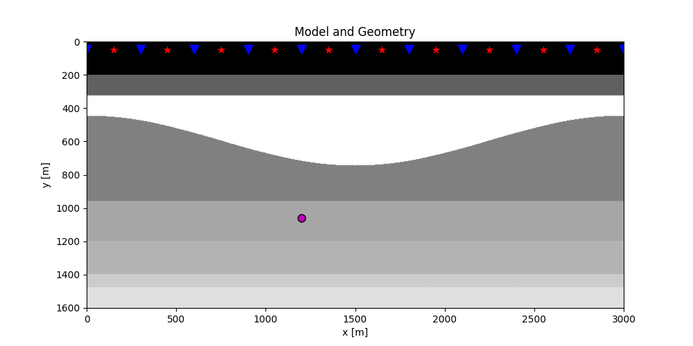
Let’s start by defining some input parameters and loading the test data
# Input parameters
inputfile = "../testdata/marchenko/input.npz"
vel = 2400.0 # velocity
toff = 0.045 # direct arrival time shift
nsmooth = 10 # time window smoothing
nfmax = 1000 # max frequency for MDC (#samples)
niter = 10 # iterations
inputdata = np.load(inputfile)
# Receivers
r = inputdata["r"]
nr = r.shape[1]
dr = r[0, 1] - r[0, 0]
# Sources
s = inputdata["s"]
ns = s.shape[1]
ds = s[0, 1] - s[0, 0]
# Virtual points
vs = inputdata["vs"]
# Density model
rho = inputdata["rho"]
z, x = inputdata["z"], inputdata["x"]
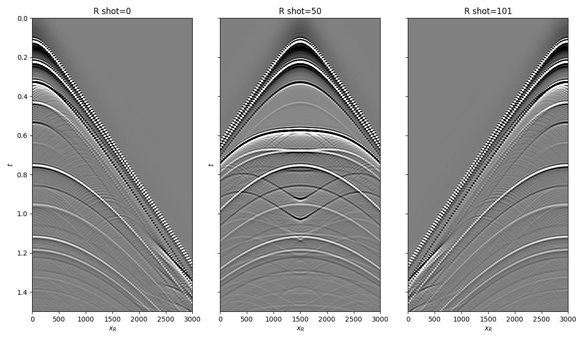
# Reflection data (R[s, r, t]) and subsurface fields
R = inputdata["R"][:, :, :-100]
R = np.swapaxes(R, 0, 1) # just because of how the data was saved
Gsub = inputdata["Gsub"][:-100]
G0sub = inputdata["G0sub"][:-100]
wav = inputdata["wav"]
wav_c = np.argmax(wav)
t = inputdata["t"][:-100]
ot, dt, nt = t[0], t[1] - t[0], len(t)
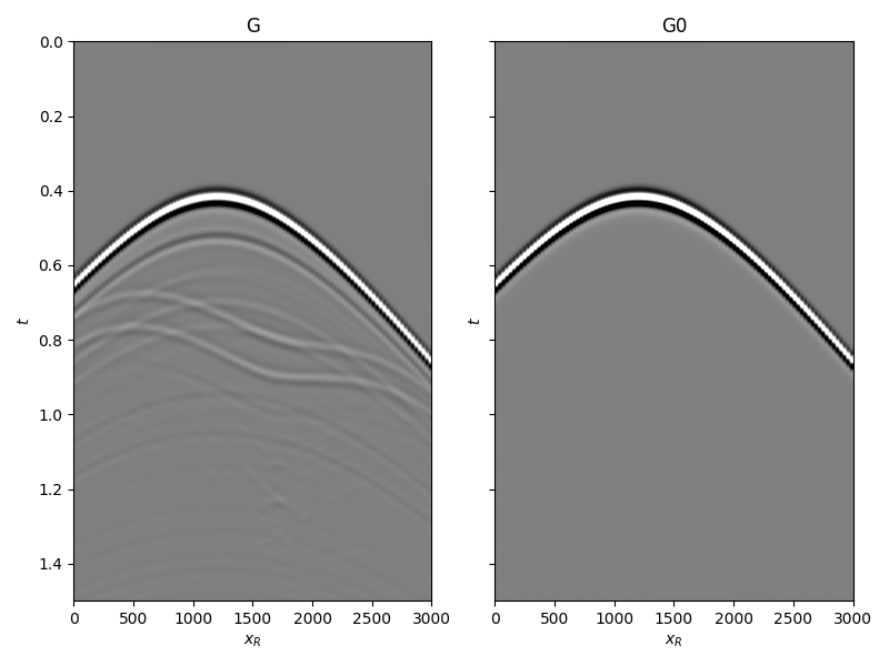
Gsub = np.apply_along_axis(convolve, 0, Gsub, wav, mode="full")
Gsub = Gsub[wav_c:][:nt]
G0sub = np.apply_along_axis(convolve, 0, G0sub, wav, mode="full")
G0sub = G0sub[wav_c:][:nt]
plt.figure(figsize=(10, 5))
plt.imshow(rho, cmap="gray", extent=(x[0], x[-1], z[-1], z[0]))
plt.scatter(s[0, 5::10], s[1, 5::10], marker="*", s=150, c="r", edgecolors="k")
plt.scatter(r[0, ::10], r[1, ::10], marker="v", s=150, c="b", edgecolors="k")
plt.scatter(vs[0], vs[1], marker=".", s=250, c="m", edgecolors="k")
plt.axis("tight")
plt.xlabel("x [m]")
plt.ylabel("y [m]")
plt.title("Model and Geometry")
plt.xlim(x[0], x[-1])
fig, axs = plt.subplots(1, 3, sharey=True, figsize=(12, 7))
axs[0].imshow(
R[0].T, cmap="gray", vmin=-1e-2, vmax=1e-2, extent=(r[0, 0], r[0, -1], t[-1], t[0])
)
axs[0].set_title("R shot=0")
axs[0].set_xlabel(r"$x_R$")
axs[0].set_ylabel(r"$t$")
axs[0].axis("tight")
axs[0].set_ylim(1.5, 0)
axs[1].imshow(
R[ns // 2].T,
cmap="gray",
vmin=-1e-2,
vmax=1e-2,
extent=(r[0, 0], r[0, -1], t[-1], t[0]),
)
axs[1].set_title("R shot=%d" % (ns // 2))
axs[1].set_xlabel(r"$x_R$")
axs[1].set_ylabel(r"$t$")
axs[1].axis("tight")
axs[1].set_ylim(1.5, 0)
axs[2].imshow(
R[-1].T, cmap="gray", vmin=-1e-2, vmax=1e-2, extent=(r[0, 0], r[0, -1], t[-1], t[0])
)
axs[2].set_title("R shot=%d" % ns)
axs[2].set_xlabel(r"$x_R$")
axs[2].axis("tight")
axs[2].set_ylim(1.5, 0)
fig.tight_layout()
fig, axs = plt.subplots(1, 2, sharey=True, figsize=(8, 6))
axs[0].imshow(
Gsub, cmap="gray", vmin=-1e6, vmax=1e6, extent=(r[0, 0], r[0, -1], t[-1], t[0])
)
axs[0].set_title("G")
axs[0].set_xlabel(r"$x_R$")
axs[0].set_ylabel(r"$t$")
axs[0].axis("tight")
axs[0].set_ylim(1.5, 0)
axs[1].imshow(
G0sub, cmap="gray", vmin=-1e6, vmax=1e6, extent=(r[0, 0], r[0, -1], t[-1], t[0])
)
axs[1].set_title("G0")
axs[1].set_xlabel(r"$x_R$")
axs[1].set_ylabel(r"$t$")
axs[1].axis("tight")
axs[1].set_ylim(1.5, 0)
fig.tight_layout()
Let’s now create an object of the
pylops.waveeqprocessing.Marchenko class and apply redatuming
for a single subsurface point vs.
# direct arrival window
trav = np.sqrt((vs[0] - r[0]) ** 2 + (vs[1] - r[1]) ** 2) / vel

MarchenkoWM = Marchenko(
    R, dt=dt, dr=dr, nfmax=nfmax, wav=wav, toff=toff, nsmooth=nsmooth
)

(
    f1_inv_minus,
    f1_inv_plus,
    p0_minus,
    g_inv_minus,
    g_inv_plus,
) = MarchenkoWM.apply_onepoint(
    trav,
    G0=G0sub.T,
    rtm=True,
    greens=True,
    dottest=True,
    **dict(iter_lim=niter, show=True)
)
g_inv_tot = g_inv_minus + g_inv_plus
Dot test passed, v^H(Opu)=405.165096396144 - u^H(Op^Hv)=405.16509639614674
Dot test passed, v^H(Opu)=172.0650756105127 - u^H(Op^Hv)=172.06507561051376

LSQR            Least-squares solution of  Ax = b
The matrix A has 282598 rows and 282598 columns
damp = 0.00000000000000e+00   calc_var =        0
atol = 1.00e-06                 conlim = 1.00e+08
btol = 1.00e-06               iter_lim =       10

   Itn      x[0]       r1norm     r2norm   Compatible    LS      Norm A   Cond A
     0  0.00000e+00   3.134e+07  3.134e+07    1.0e+00  3.3e-08
     1  0.00000e+00   1.374e+07  1.374e+07    4.4e-01  9.3e-01   1.1e+00  1.0e+00
     2  0.00000e+00   7.770e+06  7.770e+06    2.5e-01  3.9e-01   1.8e+00  2.2e+00
     3  0.00000e+00   5.750e+06  5.750e+06    1.8e-01  3.3e-01   2.1e+00  3.4e+00
     4  0.00000e+00   3.930e+06  3.930e+06    1.3e-01  3.4e-01   2.5e+00  5.1e+00
     5  0.00000e+00   3.042e+06  3.042e+06    9.7e-02  2.6e-01   2.9e+00  6.8e+00
     6  0.00000e+00   2.423e+06  2.423e+06    7.7e-02  2.2e-01   3.3e+00  8.6e+00
     7  0.00000e+00   1.675e+06  1.675e+06    5.3e-02  2.5e-01   3.6e+00  1.1e+01
     8  0.00000e+00   1.248e+06  1.248e+06    4.0e-02  2.0e-01   3.9e+00  1.3e+01
     9  0.00000e+00   1.004e+06  1.004e+06    3.2e-02  1.5e-01   4.2e+00  1.4e+01
    10  0.00000e+00   7.762e+05  7.762e+05    2.5e-02  1.8e-01   4.4e+00  1.6e+01

LSQR finished
The iteration limit has been reached

istop =       7   r1norm = 7.8e+05   anorm = 4.4e+00   arnorm = 6.1e+05
itn   =      10   r2norm = 7.8e+05   acond = 1.6e+01   xnorm  = 3.6e+07
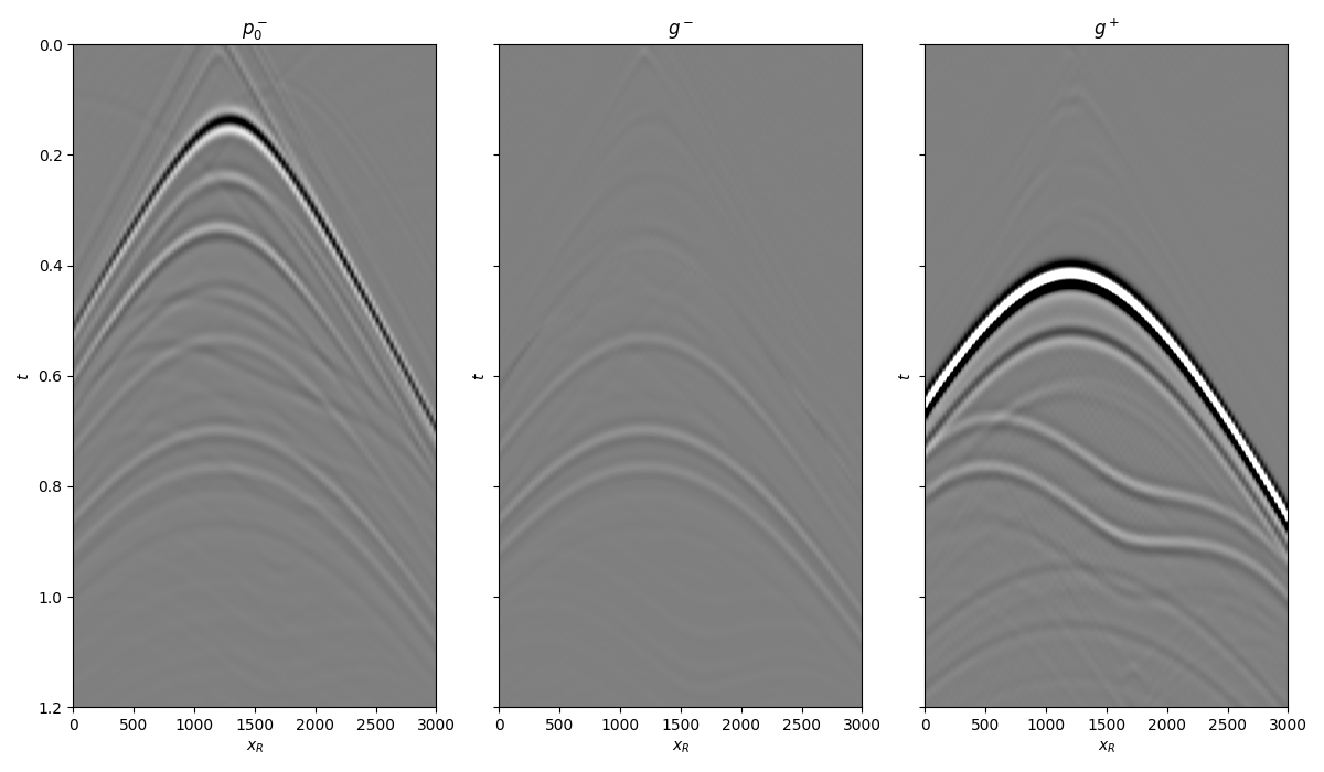
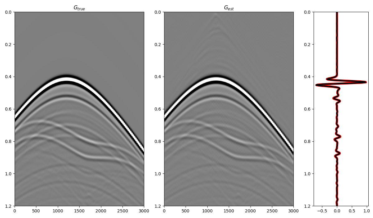
We can now compare the result of Marchenko redatuming via LSQR with standard redatuming
fig, axs = plt.subplots(1, 3, sharey=True, figsize=(12, 7))
axs[0].imshow(
    p0_minus.T,
    cmap="gray",
    vmin=-5e5,
    vmax=5e5,
    extent=(r[0, 0], r[0, -1], t[-1], -t[-1]),
)
axs[0].set_title(r"$p_0^-$")
axs[0].set_xlabel(r"$x_R$")
axs[0].set_ylabel(r"$t$")
axs[0].axis("tight")
axs[0].set_ylim(1.2, 0)
axs[1].imshow(
    g_inv_minus.T,
    cmap="gray",
    vmin=-5e5,
    vmax=5e5,
    extent=(r[0, 0], r[0, -1], t[-1], -t[-1]),
)
axs[1].set_title(r"$g^-$")
axs[1].set_xlabel(r"$x_R$")
axs[1].set_ylabel(r"$t$")
axs[1].axis("tight")
axs[1].set_ylim(1.2, 0)
axs[2].imshow(
    g_inv_plus.T,
    cmap="gray",
    vmin=-5e5,
    vmax=5e5,
    extent=(r[0, 0], r[0, -1], t[-1], -t[-1]),
)
axs[2].set_title(r"$g^+$")
axs[2].set_xlabel(r"$x_R$")
axs[2].set_ylabel(r"$t$")
axs[2].axis("tight")
axs[2].set_ylim(1.2, 0)
fig.tight_layout()

fig = plt.figure(figsize=(12, 7))
ax1 = plt.subplot2grid((1, 5), (0, 0), colspan=2)
ax2 = plt.subplot2grid((1, 5), (0, 2), colspan=2)
ax3 = plt.subplot2grid((1, 5), (0, 4))
ax1.imshow(
    Gsub, cmap="gray", vmin=-5e5, vmax=5e5, extent=(r[0, 0], r[0, -1], t[-1], t[0])
)
ax1.set_title(r"$G_{true}$")
axs[0].set_xlabel(r"$x_R$")
axs[0].set_ylabel(r"$t$")
ax1.axis("tight")
ax1.set_ylim(1.2, 0)
ax2.imshow(
    g_inv_tot.T,
    cmap="gray",
    vmin=-5e5,
    vmax=5e5,
    extent=(r[0, 0], r[0, -1], t[-1], -t[-1]),
)
ax2.set_title(r"$G_{est}$")
axs[1].set_xlabel(r"$x_R$")
axs[1].set_ylabel(r"$t$")
ax2.axis("tight")
ax2.set_ylim(1.2, 0)
ax3.plot(Gsub[:, nr // 2] / Gsub.max(), t, "r", lw=5)
ax3.plot(g_inv_tot[nr // 2, nt - 1 :] / g_inv_tot.max(), t, "k", lw=3)
ax3.set_ylim(1.2, 0)
fig.tight_layout()
Note that Marchenko redatuming can also be applied simultaneously
to multiple subsurface points. Use
pylops.waveeqprocessing.Marchenko.apply_multiplepoints instead of
pylops.waveeqprocessing.Marchenko.apply_onepoint.
Total running time of the script: (0 minutes 4.005 seconds)