pylops.signalprocessing.Seislet
- class pylops.signalprocessing.Seislet(slopes, sampling=(1.0, 1.0), level=None, kind='haar', inv=False, dtype='float64', name='S')[source]
Two dimensional Seislet operator.
Apply 2D-Seislet Transform to an input array given an estimate of its local
slopes. In forward mode, the input array is reshaped into a two-dimensional array of size \(n_x \times n_t\) and the transform is performed along the first (spatial) axis (see Notes for more details).- Parameters:
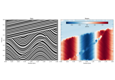
- slopes
numpy.ndarray Slope field of size \(n_x \times n_t\)
- sampling
tuple, optional Sampling steps in x- and t-axis.
- level
int, optional Number of scaling levels (must be >=0).
- kind
str, optional Basis function used for predict and update steps:
haarorlinear.- inv
int, optional Apply inverse transform when invoking the adjoint (
True) or not (False). Note that in some scenario it may be more appropriate to use the exact inverse as adjoint of the Seislet operator even if this is not an orthogonal operator and the dot-test would not be satisfied (see Notes for details). Otherwise, the user can access the inverse directly as method of this class.- dtype
str, optional Type of elements in input array.
- name
str, optional Added in version 2.0.0.
Name of operator (to be used by
pylops.utils.describe.describe)
- slopes
- Attributes:
- predict
callable Function used for the predict step.
- padop
pylops.basicoperators.Pad Padding operator used to make the number of traces multiple of \(2^{level}\).
- nx
int Number of traces after padding.
- nt
int Number of samples per trace.
- dx
float Sampling step in x-axis.
- dt
float Sampling step in t-axis.
- levels_size
int Number of traces for each level.
- levels_cum
int Cumulative number of traces up to each level.
- slopes
numpy.ndarray Padded slope field.
- dims
tuple Shape of the array after the adjoint, but before flattening.
For example,
x_reshaped = (Op.H * y.ravel()).reshape(Op.dims).- dimsd
tuple Shape of the array after the forward, but before flattening.
For example,
y_reshaped = (Op * x.ravel()).reshape(Op.dimsd).- shape
tuple Operator shape.
- predict
- Raises:
- NotImplementedError
If
kindis different from haar or linear- ValueError
If
samplinghas more or less than two elements.
Notes
The Seislet transform [1] is implemented using the lifting scheme.
In its simplest form (i.e., corresponding to the Haar basis function for the Wavelet transform) the input dataset is separated into even (\(\mathbf{e}\)) and odd (\(\mathbf{o}\)) traces. Even traces are used to forward predict the odd traces using local slopes and the new odd traces (also referred to as residual) is defined as:
\[\mathbf{o}^{i+1} = \mathbf{r}^i = \mathbf{o}^i - P(\mathbf{e}^i)\]where \(P = P^+\) is the slope-based forward prediction operator (which is here implemented as a sinc-based resampling). The residual is then updated and summed to the even traces to obtain the new even traces (also referred to as coarse representation):
\[\mathbf{e}^{i+1} = \mathbf{c}^i = \mathbf{e}^i + U(\mathbf{o}^{i+1})\]where \(U = P^- / 2\) is the update operator which performs a slope-based backward prediction. At this point \(\mathbf{e}^{i+1}\) becomes the new data and the procedure is repeated level times (at maximum until \(\mathbf{e}^{i+1}\) is a single trace. The Seislet transform is effectively composed of all residuals and the coarsest data representation.
In the inverse transform the two operations are reverted. Starting from the coarsest scale data representation \(\mathbf{c}\) and residual \(\mathbf{r}\), the even and odd parts of the previous scale are reconstructed as:
\[\mathbf{e}^i = \mathbf{c}^i - U(\mathbf{r}^i) = \mathbf{e}^{i+1} - U(\mathbf{o}^{i+1})\]and:
\[\mathbf{o}^i = \mathbf{r}^i + P(\mathbf{e}^i) = \mathbf{o}^{i+1} + P(\mathbf{e}^i)\]A new data is formed by interleaving \(\mathbf{e}^i\) and \(\mathbf{o}^i\) and the procedure repeated until the new data as the same number of traces as the original one.
Finally the adjoint operator can be easily derived by writing the lifting scheme in a matricial form:
\[\begin{split}\begin{bmatrix} \mathbf{r}_1 \\ \mathbf{r}_2 \\ \vdots \\ \mathbf{r}_N \\ \mathbf{c}_1 \\ \mathbf{c}_2 \\ \vdots \\ \mathbf{c}_N \end{bmatrix} = \begin{bmatrix} \mathbf{I} & \mathbf{0} & \ldots & \mathbf{0} & -\mathbf{P} & \mathbf{0} & \ldots & \mathbf{0} \\ \mathbf{0} & \mathbf{I} & \ldots & \mathbf{0} & \mathbf{0} & -\mathbf{P} & \ldots & \mathbf{0} \\ \vdots & \vdots & \ddots & \vdots & \vdots & \vdots & \ddots & \vdots \\ \mathbf{0} & \mathbf{0} & \ldots & \mathbf{I} & \mathbf{0} & \mathbf{0} & \ldots & -\mathbf{P} \\ \mathbf{U} & \mathbf{0} & \ldots & \mathbf{0} & \mathbf{I}-\mathbf{UP} & \mathbf{0} & \ldots & \mathbf{0} \\ \mathbf{0} & \mathbf{U} & \ldots & \mathbf{0} & \mathbf{0} & \mathbf{I}-\mathbf{UP} & \ldots & \mathbf{0} \\ \vdots & \vdots & \ddots & \vdots & \vdots & \vdots & \ddots & \vdots \\ \mathbf{0} & \mathbf{0} & \ldots & \mathbf{U} & \mathbf{0} & \mathbf{0} & \ldots & \mathbf{I}-\mathbf{UP} \end{bmatrix} \begin{bmatrix} \mathbf{o}_1 \\ \mathbf{o}_2 \\ \vdots \\ \mathbf{o}_N \\ \mathbf{e}_1 \\ \mathbf{e}_2 \\ \vdots \\ \mathbf{e}_N \end{bmatrix}\end{split}\]Transposing the operator leads to:
\[\begin{split}\begin{bmatrix} \mathbf{o}_1 \\ \mathbf{o}_2 \\ \vdots \\ \mathbf{o}_N \\ \mathbf{e}_1 \\ \mathbf{e}_2 \\ \vdots \\ \mathbf{e}_N \end{bmatrix} = \begin{bmatrix} \mathbf{I} & \mathbf{0} & \ldots & \mathbf{0} & -\mathbf{U^T} & \mathbf{0} & \ldots & \mathbf{0} \\ \mathbf{0} & \mathbf{I} & \ldots & \mathbf{0} & \mathbf{0} & -\mathbf{U^T} & \ldots & \mathbf{0} \\ \vdots & \vdots & \ddots & \vdots & \vdots & \vdots & \ddots & \vdots \\ \mathbf{0} & \mathbf{0} & \ldots & \mathbf{I} & \mathbf{0} & \mathbf{0} & \ldots & -\mathbf{U^T} \\ \mathbf{P^T} & \mathbf{0} & \ldots & \mathbf{0} & \mathbf{I}-\mathbf{P^T U^T} & \mathbf{0} & \ldots & \mathbf{0} \\ \mathbf{0} & \mathbf{P^T} & \ldots & \mathbf{0} & \mathbf{0} & \mathbf{I}-\mathbf{P^T U^T} & \ldots & \mathbf{0} \\ \vdots & \vdots & \ddots & \vdots & \vdots & \vdots & \ddots & \vdots \\ \mathbf{0} & \mathbf{0} & \ldots & \mathbf{P^T} & \mathbf{0} & \mathbf{0} & \ldots & \mathbf{I}-\mathbf{P^T U^T} \end{bmatrix} \begin{bmatrix} \mathbf{r}_1 \\ \mathbf{r}_2 \\ \vdots \\ \mathbf{r}_N \\ \mathbf{c}_1 \\ \mathbf{c}_2 \\ \vdots \\ \mathbf{c}_N \end{bmatrix}\end{split}\]which can be written more easily in the following two steps:
\[\mathbf{o} = \mathbf{r} + \mathbf{U}^H\mathbf{c}\]and:
\[\mathbf{e} = \mathbf{c} - \mathbf{P}^H(\mathbf{r} + \mathbf{U}^H(\mathbf{c})) = \mathbf{c} - \mathbf{P}^H\mathbf{o}\]Similar derivations follow for more complex wavelet bases.
[1]Fomel, S., Liu, Y., “Seislet transform and seislet frame”, Geophysics, 75, no. 3, V25-V38. 2010.
Methods
__init__(slopes[, sampling, level, kind, ...])adjoint()apply_columns(cols)Apply subset of columns of operator
cond([uselobpcg])Condition number of linear operator.
conj()Complex conjugate operator
div(y[, niter, densesolver])Solve the linear problem \(\mathbf{y}=\mathbf{A}\mathbf{x}\).
dot(x)Matrix-matrix or matrix-vector multiplication.
eigs([neigs, symmetric, niter, uselobpcg])Most significant eigenvalues of linear operator.
inverse(x)matmat(X)Matrix-matrix multiplication.
matvec(x)Matrix-vector multiplication.
reset_count()Reset counters
rmatmat(X)Matrix-matrix multiplication.
rmatvec(x)Adjoint matrix-vector multiplication.
todense([backend])Return dense matrix.
toimag([forw, adj])Imag operator
toreal([forw, adj])Real operator
tosparse()Return sparse matrix.
trace([neval, method, backend])Trace of linear operator.
transpose()