pylops.waveeqprocessing.MDC
- pylops.waveeqprocessing.MDC(G, nt, nv, dt=1.0, dr=1.0, twosided=True, fftengine='numpy', saveGt=True, conj=False, usematmul=False, prescaled=False, name='M', **kwargs_fft)[source]
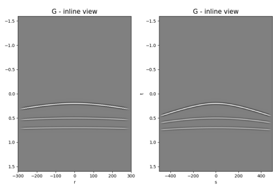
Multi-dimensional convolution.
Apply multi-dimensional convolution between two datasets. Model and data should be provided after flattening 2- or 3-dimensional arrays of size \([n_t \times n_r \;(\times n_{vs})]\) and \([n_t \times n_s \;(\times n_{vs})]\) (or \(2n_t-1\) for
twosided=True), respectively.- Parameters:
- G
numpy.ndarray Multi-dimensional convolution kernel in frequency domain of size \([n_{f_\text{max}} \times n_s \times n_r]\)
- nt
int Number of samples along time axis for model and data (note that this must be equal to \(2n_t-1\) when working with
twosided=True.- nv
int Number of samples along virtual source axis
- dt
float, optional Sampling of time integration axis \(\Delta t\)
- dr
float, optional Sampling of receiver integration axis \(\Delta r\)
- twosided
bool, optional MDC operator has both negative and positive time (
True) or only positive (False)- fftengine
str, optional Engine used for fft computation (
numpy,scipyorfftw)- saveGt
bool, optional Save
GandG.Hto speed up the computation of adjoint ofpylops.signalprocessing.Fredholm1(True) or createG.Hon-the-fly (False) Note thatsaveGt=Truewill be faster but double the amount of required memory- conj
str, optional Perform Fredholm integral computation with complex conjugate of
G- usematmul
bool, optional Use
numpy.matmul(True) or for-loop withnumpy.dot(False) inpylops.signalprocessing.Fredholm1operator. Refer to Fredholm1 documentation for details.- prescaled
bool, optional Apply scaling to kernel (
False) or not (False) when performing spatial and temporal summations. In caseprescaled=True, the kernel is assumed to have been pre-scaled when passed to the MDC routine.- name
str, optional Added in version 2.0.0.
Name of operator (to be used by
pylops.utils.describe.describe)- **kwargs_fft
Added in version 2.6.0.
Arbitrary keyword arguments to be passed to the selected fft method
- G
- Returns:
- MOp
pylops.LinearOperator Multi-dimensional convolution operator.
- MOp
- Raises:
- ValueError
If
ntis even andtwosided=True
See also
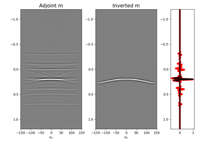
MDDMulti-dimensional deconvolution
Notes
The so-called multi-dimensional convolution (MDC) is a chained operator [1]. It is composed of a forward Fourier transform, a multi-dimensional integration, and an inverse Fourier transform:
\[y(t, s, v) = \mathscr{F}^{-1} \Big( \int_S G(f, s, r) \mathscr{F}(x(t, r, v))\,\mathrm{d}r \Big)\]which is discretized as follows:
\[y(t, s, v) = \sqrt{n_t} \Delta t \Delta r\mathscr{F}^{-1} \Big( \sum_{i_r=0}^{n_r} G(f, s, i_r) \mathscr{F}(x(t, i_r, v)) \Big)\]where \(\sqrt{n_t} \Delta t \Delta r\) is not applied if
prescaled=True.This operation can be discretized and performed by means of a linear operator
\[\mathbf{D}= \mathbf{F}^H \mathbf{G} \mathbf{F}\]where \(\mathbf{F}\) is the Fourier transform applied along the time axis and \(\mathbf{G}\) is the multi-dimensional convolution kernel.
[1]Wapenaar, K., van der Neut, J., Ruigrok, E., Draganov, D., Hunziker, J., Slob, E., Thorbecke, J., and Snieder, R., “Seismic interferometry by crosscorrelation and by multi-dimensional deconvolution: a systematic comparison”, Geophysical Journal International, vol. 185, pp. 1335-1364. 2011.