Note
Go to the end to download the full example code.
PhaseShift operator
This example shows how to use the pylops.waveeqprocessing.PhaseShift
operator to perform frequency-wavenumber shift of an input multi-dimensional
signal. Such a procedure is applied in a variety of disciplines including
geophysics, medical imaging and non-destructive testing.
import matplotlib.pyplot as plt
import numpy as np

import pylops

plt.close("all")
Let’s first create a synthetic dataset composed of a number of hyperbolas
par = {
    "ox": -300,
    "dx": 20,
    "nx": 31,
    "oy": -200,
    "dy": 20,
    "ny": 21,
    "ot": 0,
    "dt": 0.004,
    "nt": 201,
    "f0": 20,
    "nfmax": 210,
}

# Create axis
t, t2, x, y = pylops.utils.seismicevents.makeaxis(par)

# Create wavelet
wav = pylops.utils.wavelets.ricker(np.arange(41) * par["dt"], f0=par["f0"])[0]

vrms = [900, 1300, 1800]
t0 = [0.2, 0.3, 0.6]
amp = [1.0, 0.6, -2.0]

_, m = pylops.utils.seismicevents.hyperbolic2d(x, t, t0, vrms, amp, wav)
We can now apply a taper at the edges and also pad the input to avoid artifacts during the phase shift
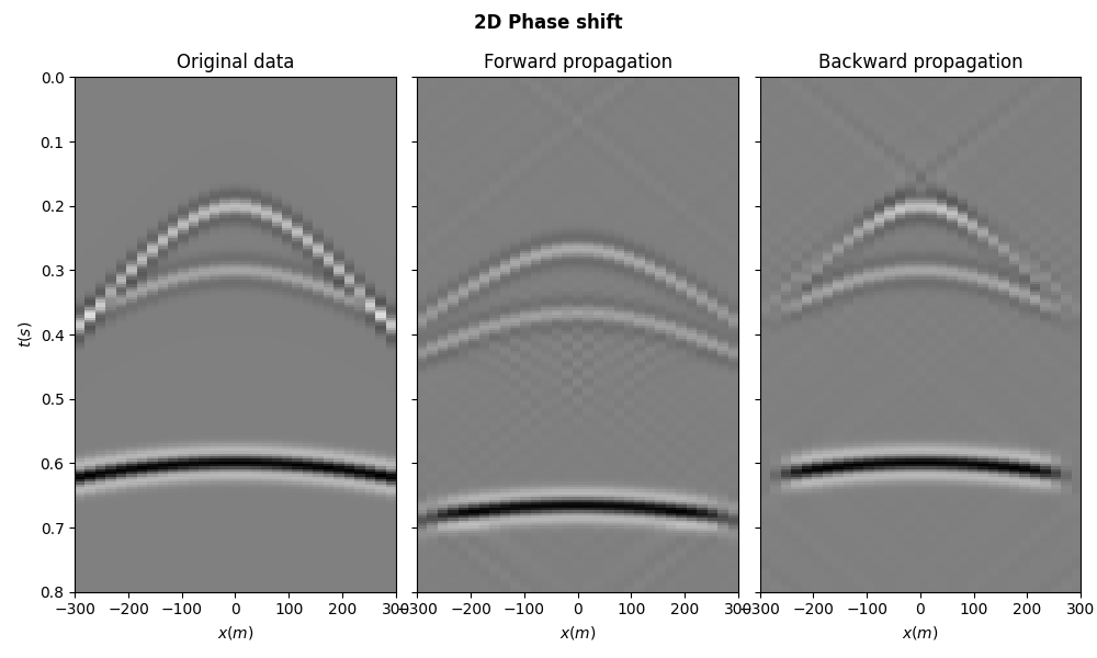
We perform now forward propagation in a constant velocity \(v=2000\) for a depth of \(z_{prop} = 100 m\). We should expect the hyperbolas to move forward in time and become flatter.
vel = 1500.0
zprop = 100
freq = np.fft.rfftfreq(par["nt"], par["dt"])
kx = np.fft.fftshift(np.fft.fftfreq(par["nx"] + 2 * pad, par["dx"]))
Pop = pylops.waveeqprocessing.PhaseShift(vel, zprop, par["nt"], freq, kx)

mdown = Pop * mpad.T.ravel()
We now take the forward propagated wavefield and apply backward propagation, which is in this case simply the adjoint of our operator. We should expect the hyperbolas to move backward in time and show the same traveltime as the original dataset. Of course, as we are only performing the adjoint operation we should expect some small differences between this wavefield and the input dataset.
mup = Pop.H * mdown.ravel()

mdown = np.real(mdown.reshape(par["nt"], par["nx"] + 2 * pad)[:, pad:-pad])
mup = np.real(mup.reshape(par["nt"], par["nx"] + 2 * pad)[:, pad:-pad])

fig, axs = plt.subplots(1, 3, figsize=(10, 6), sharey=True)
fig.suptitle("2D Phase shift", fontsize=12, fontweight="bold")
axs[0].imshow(
    m.T,
    aspect="auto",
    interpolation="nearest",
    vmin=-2,
    vmax=2,
    cmap="gray",
    extent=(x.min(), x.max(), t.max(), t.min()),
)
axs[0].set_xlabel(r"$x(m)$")
axs[0].set_ylabel(r"$t(s)$")
axs[0].set_title("Original data")
axs[1].imshow(
    mdown,
    aspect="auto",
    interpolation="nearest",
    vmin=-2,
    vmax=2,
    cmap="gray",
    extent=(x.min(), x.max(), t.max(), t.min()),
)
axs[1].set_xlabel(r"$x(m)$")
axs[1].set_title("Forward propagation")
axs[2].imshow(
    mup,
    aspect="auto",
    interpolation="nearest",
    vmin=-2,
    vmax=2,
    cmap="gray",
    extent=(x.min(), x.max(), t.max(), t.min()),
)
axs[2].set_xlabel(r"$x(m)$")
axs[2].set_title("Backward propagation")
plt.tight_layout()
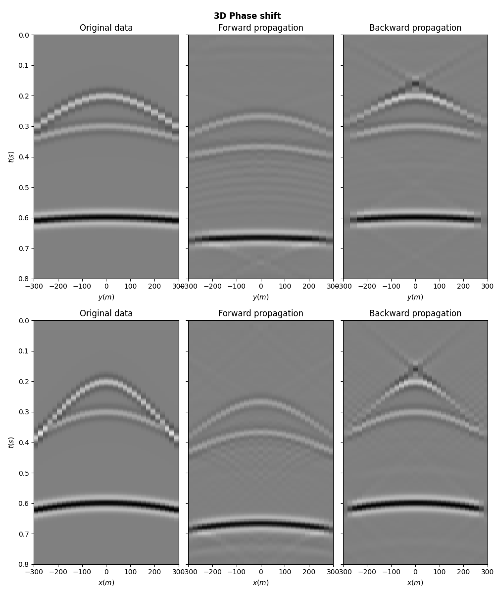
Finally we perform the same for a 3-dimensional signal
_, m = pylops.utils.seismicevents.hyperbolic3d(x, y, t, t0, vrms, vrms, amp, wav)

pad = 11
taper = pylops.utils.tapers.taper3d(par["nt"], (par["ny"], par["nx"]), (3, 3))
mpad = np.pad(m * taper, ((pad, pad), (pad, pad), (0, 0)), mode="constant")

kx = np.fft.fftshift(np.fft.fftfreq(par["nx"] + 2 * pad, par["dx"]))
ky = np.fft.fftshift(np.fft.fftfreq(par["ny"] + 2 * pad, par["dy"]))
Pop = pylops.waveeqprocessing.PhaseShift(vel, zprop, par["nt"], freq, kx, ky)

mdown = Pop * mpad.transpose(2, 1, 0).ravel()

mup = Pop.H * mdown.ravel()

mdown = np.real(
    mdown.reshape(par["nt"], par["nx"] + 2 * pad, par["ny"] + 2 * pad)[
        :, pad:-pad, pad:-pad
    ]
)
mup = np.real(
    mup.reshape(par["nt"], par["nx"] + 2 * pad, par["ny"] + 2 * pad)[
        :, pad:-pad, pad:-pad
    ]
)

fig, axs = plt.subplots(2, 3, figsize=(10, 12), sharey=True)
fig.suptitle("3D Phase shift", fontsize=12, fontweight="bold")
axs[0][0].imshow(
    m[:, par["nx"] // 2].T,
    aspect="auto",
    interpolation="nearest",
    vmin=-2,
    vmax=2,
    cmap="gray",
    extent=(x.min(), x.max(), t.max(), t.min()),
)
axs[0][0].set_xlabel(r"$y(m)$")
axs[0][0].set_ylabel(r"$t(s)$")
axs[0][0].set_title("Original data")
axs[0][1].imshow(
    mdown[:, par["nx"] // 2],
    aspect="auto",
    interpolation="nearest",
    vmin=-2,
    vmax=2,
    cmap="gray",
    extent=(x.min(), x.max(), t.max(), t.min()),
)
axs[0][1].set_xlabel(r"$y(m)$")
axs[0][1].set_title("Forward propagation")
axs[0][2].imshow(
    mup[:, par["nx"] // 2],
    aspect="auto",
    interpolation="nearest",
    vmin=-2,
    vmax=2,
    cmap="gray",
    extent=(x.min(), x.max(), t.max(), t.min()),
)
axs[0][2].set_xlabel(r"$y(m)$")
axs[0][2].set_title("Backward propagation")
axs[1][0].imshow(
    m[par["ny"] // 2].T,
    aspect="auto",
    interpolation="nearest",
    vmin=-2,
    vmax=2,
    cmap="gray",
    extent=(x.min(), x.max(), t.max(), t.min()),
)
axs[1][0].set_xlabel(r"$x(m)$")
axs[1][0].set_ylabel(r"$t(s)$")
axs[1][0].set_title("Original data")
axs[1][1].imshow(
    mdown[:, :, par["ny"] // 2],
    aspect="auto",
    interpolation="nearest",
    vmin=-2,
    vmax=2,
    cmap="gray",
    extent=(x.min(), x.max(), t.max(), t.min()),
)
axs[1][1].set_xlabel(r"$x(m)$")
axs[1][1].set_title("Forward propagation")
axs[1][2].imshow(
    mup[:, :, par["ny"] // 2],
    aspect="auto",
    interpolation="nearest",
    vmin=-2,
    vmax=2,
    cmap="gray",
    extent=(x.min(), x.max(), t.max(), t.min()),
)
axs[1][2].set_xlabel(r"$x(m)$")
axs[1][2].set_title("Backward propagation")
plt.tight_layout()
Total running time of the script: (0 minutes 0.858 seconds)