pylops.waveeqprocessing.BlendingContinuous

class pylops.waveeqprocessing.BlendingContinuous(nt, nr, ns, dt, times, shiftall=False, nttot=None, dtype='float64', name='B', **kwargs_fft)

Continuous blending operator

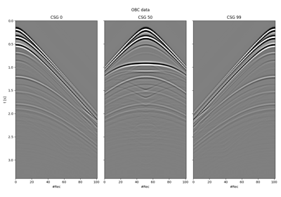
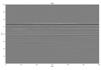
Blend seismic shot gathers in continuous mode based on pre-defined sequence of firing times. The size of input model vector must be \(n_s \times n_r \times n_t\), whilst the size of the data vector is \(n_r \times n_{t,tot}\).

Parameters:

ntint

Number of time samples

nrint

Number of receivers

nsint

Number of sources

dtfloat

Time sampling in seconds

timesnumpy.ndarray

Absolute ignition times for each source

shiftallbool, optional

Shift all shots together (True) or one at the time (False). Defaults to shiftall=False (original implementation), however shiftall=True should be preferred when nr is small.

nttotint

Total number of time samples in blended data (if None, computed internally based on the the maximum ignition time in times)

dtypestr, optional

Operator dtype

namestr, optional

Name of operator (to be used by pylops.utils.describe.describe)

**kwargs_fft

Added in version 2.6.0.

Arbitrary keyword arguments to be passed to the Shift operator

Attributes:

PadOppylops.basicoperators.Pad

Padding operator used to add one zero at the end of each shot gather to avoid boundary effects when shifting

shiftslist or numpy.ndarray

Integer part of the time shifts (in number of samples)

ShiftOpslist of pylops.signalprocessing.Shift or pylops.signalprocessing.Shift

Shift operator(s) used to apply the fractional part of the time shifts

dimstuple

Shape of the array after the adjoint, but before flattening.

For example, x_reshaped = (Op.H * y.ravel()).reshape(Op.dims).

dimsdtuple

Shape of the array after the forward, but before flattening.

For example, y_reshaped = (Op * x.ravel()).reshape(Op.dimsd).

shapetuple

Operator shape.

Notes

Simultaneous shooting or blending is the process of acquiring seismic data firing consecutive sources at short time intervals (shorter than the time requires for all significant waves to come back from the Earth interior).

Continuous blending refers to an acquisition scenario where a source towed behind a single vessel is fired at irregular time intervals (times) to create a continuous recording whose modelling operator is

\[\Phi = [\Phi_1, \Phi_2, ..., \Phi_N]\]

where each \(\Phi_i\) operator applies a time-shift equal to the absolute ignition time provided in the variable times.

Methods

__init__(nt, nr, ns, dt, times[, shiftall, ...])
adjoint()
apply_columns(cols)	Apply subset of columns of operator
cond([uselobpcg])	Condition number of linear operator.
conj()	Complex conjugate operator
div(y[, niter, densesolver])	Solve the linear problem \(\mathbf{y}=\mathbf{A}\mathbf{x}\).
dot(x)	Matrix-matrix or matrix-vector multiplication.
eigs([neigs, symmetric, niter, uselobpcg])	Most significant eigenvalues of linear operator.
matmat(X)	Matrix-matrix multiplication.
matvec(x)	Matrix-vector multiplication.
reset_count()	Reset counters
rmatmat(X)	Matrix-matrix multiplication.
rmatvec(x)	Adjoint matrix-vector multiplication.
todense([backend])	Return dense matrix.
toimag([forw, adj])	Imag operator
toreal([forw, adj])	Real operator
tosparse()	Return sparse matrix.
trace([neval, method, backend])	Trace of linear operator.
transpose()

Examples using pylops.waveeqprocessing.BlendingContinuous

Blending

Blending

18. Deblending

18. Deblending