PWD-based slope estimation and structural smoothing

This example shows how to estimate local slopes of a two-dimensional array using the Plane-Wave Destruction (PWD [1]) algorithm via pylops.utils.signalprocessing.pwd_slope_estimate; such slopes are then used as a guide to smooth a noise realization following the structural dips of the input data via the pylops.signalprocessing.PWSmoother2D.

[1]

Fomel, S., “Applications of plane-wave destruction filters”, Geophysics. 2002.

from functools import partial

import matplotlib.pyplot as plt
import numpy as np
from mpl_toolkits.axes_grid1 import make_axes_locatable

import pylops
from pylops.signalprocessing import PWSmoother2D
from pylops.utils.signalprocessing import pwd_slope_estimate, slope_estimate

plt.close("all")
np.random.seed(10)


def create_colorbar(im, ax):
    divider = make_axes_locatable(ax)
    cax = divider.append_axes("right", size="5%", pad=0.1)
    cb = fig.colorbar(im, cax=cax, orientation="vertical")
    return cax, cb

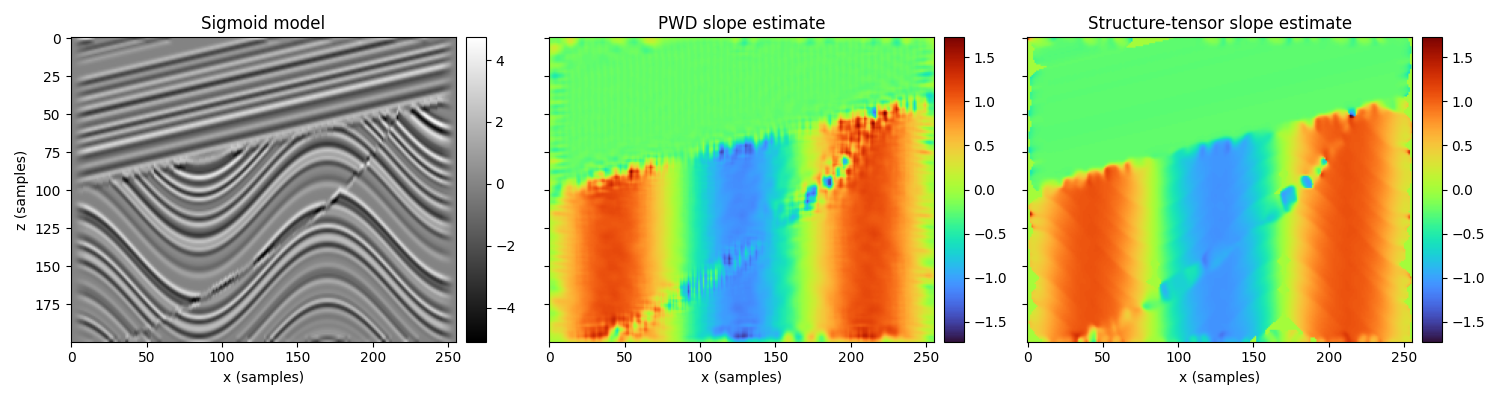
Sigmoid model

To start we import the same 2D image that we used in the seislet transform example. This image contains curved reflectors that we will try to follow during the smoothing operation.

inputfile = "../testdata/sigmoid.npz"

sigmoid = 1e3 * np.load(inputfile)["sigmoid"].T
nz, nx = sigmoid.shape

Slope estimation comparison between PWD and Structure Tensor

Next, slopes are estimated using both the plane-wave destruction and the structure-tensor algorithms. Both algorithms return slopes in samples per trace.

pwd_slope = pwd_slope_estimate(
    sigmoid,
    niter=5,
    liter=20,
    order=2,
    smoothing="triangle",
    nsmooth=(12, 12),
    damp=6e-4,
).astype(np.float32)

st_slope, _ = slope_estimate(
    sigmoid,
    dz=1.0,
    dx=1.0,
    smooth=2.0,
    eps=2e-3,
    dips=False,
)
# Defined with z-point upwards, reverse the convention
st_slope *= -1
st_slope = st_slope.astype(np.float32)

fig, ax = plt.subplots(1, 3, figsize=(15, 4), sharey=True)

im0 = ax[0].imshow(sigmoid, aspect="auto", cmap="gray")
create_colorbar(im0, ax=ax[0])
ax[0].set_title("Sigmoid model")

v = np.max(np.abs(pwd_slope))
im1 = ax[1].imshow(pwd_slope, aspect="auto", cmap="turbo", vmin=-v, vmax=v)
ax[1].set_title("PWD slope estimate")
create_colorbar(im1, ax=ax[1])

im2 = ax[2].imshow(st_slope, aspect="auto", cmap="turbo", vmin=-v, vmax=v)
ax[2].set_title("Structure-tensor slope estimate")
create_colorbar(im2, ax=ax[2])

for a in ax:
    a.set_xlabel("x (samples)")
ax[0].set_ylabel("z (samples)")
fig.tight_layout()

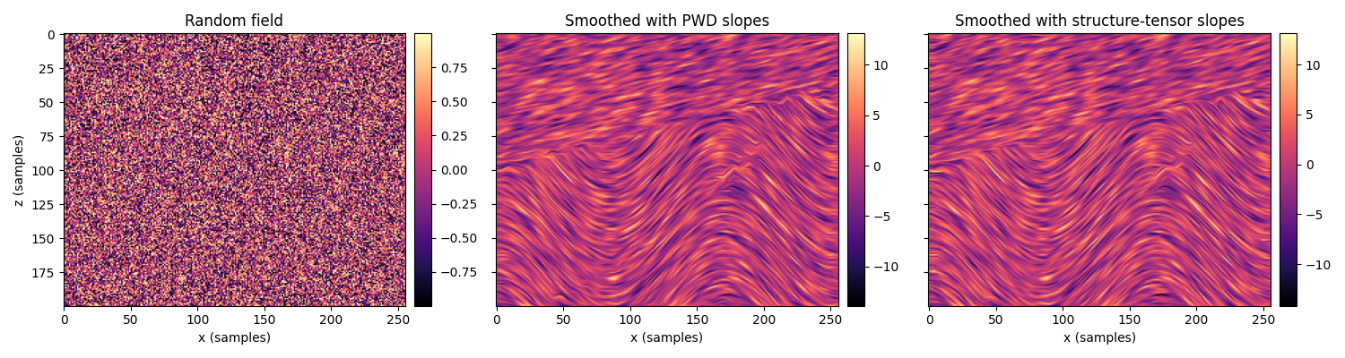
Structure-aligned smoothing via local slopes

The estimated slopes are finally used by the pylops.signalprocessing.PWSmoother2D operator to perform structure-aligned smoothing of a random noise realization. Note that this operator is defined as the composition of a pylops.signalprocessing.PWSprayer2D operator and its adjoint (i.e., Sprayer.T @ Sprayer) and therefore it is a symmetric operator.

noise = np.random.uniform(-1.0, 1.0, size=(nz, nx)).astype(np.float32)

radius = 6
alpha = 0.7

SOp_pwd = PWSmoother2D(
    dims=(nz, nx), sigma=pwd_slope, radius=radius, alpha=alpha, dtype="float32"
)
smooth_pwd = SOp_pwd @ noise

SOp_st = PWSmoother2D(
    dims=(nz, nx), sigma=st_slope, radius=radius, alpha=alpha, dtype="float32"
)
smooth_st = SOp_st @ noise

fig, ax = plt.subplots(1, 3, figsize=(15, 4), sharey=True)

im0 = ax[0].imshow(noise, aspect="auto", cmap="magma")
ax[0].set_title("Random field")
create_colorbar(im0, ax=ax[0])

im1 = ax[1].imshow(smooth_pwd, aspect="auto", cmap="magma")
ax[1].set_title("Smoothed with PWD slopes")
create_colorbar(im1, ax=ax[1])

im2 = ax[2].imshow(smooth_st, aspect="auto", cmap="magma")
ax[2].set_title("Smoothed with structure-tensor slopes")
create_colorbar(im2, ax=ax[2])

for a in ax:
    a.set_xlabel("x (samples)")
ax[0].set_ylabel("z (samples)")
fig.tight_layout()

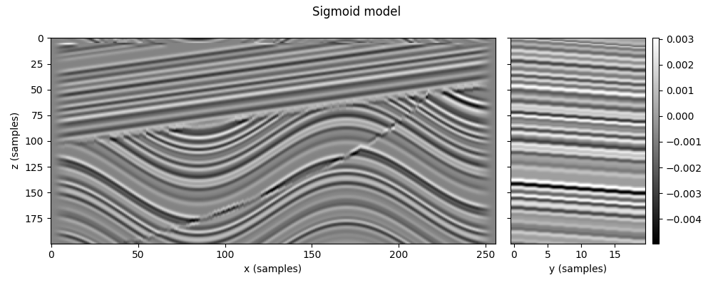
3D Extension

Finally, we show here how the PWD slope estimation and smoothing algorithms can be easily extended to 3D data. We start by generating a 3D synthetic volume composed of 10 adjacent 2D sigmoid slices shifted in depth.

ny = 20

sigmoid3d = np.zeros((ny, nz, nx), dtype=sigmoid.dtype)
for i in range(ny):
    sigmoid3d[i, ...] = np.roll(sigmoid / 1e3, i // 2, axis=0)

fig, ax = plt.subplots(1, 2, figsize=(10, 4), sharey=True, width_ratios=(3, 1))
fig.suptitle("Sigmoid model")
ax[0].imshow(sigmoid3d[ny // 2], aspect="auto", cmap="gray")
ax[0].set_ylabel("z (samples)")
ax[0].set_xlabel("x (samples)")
im1 = ax[1].imshow(sigmoid3d[..., nx // 2].T, aspect="auto", cmap="gray")
ax[1].set_xlabel("y (samples)")
create_colorbar(im1, ax=ax[1])
fig.tight_layout()

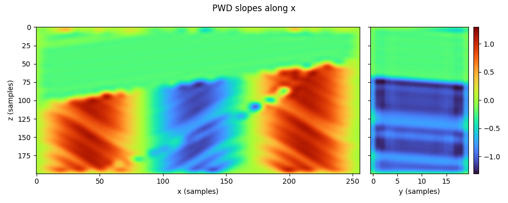
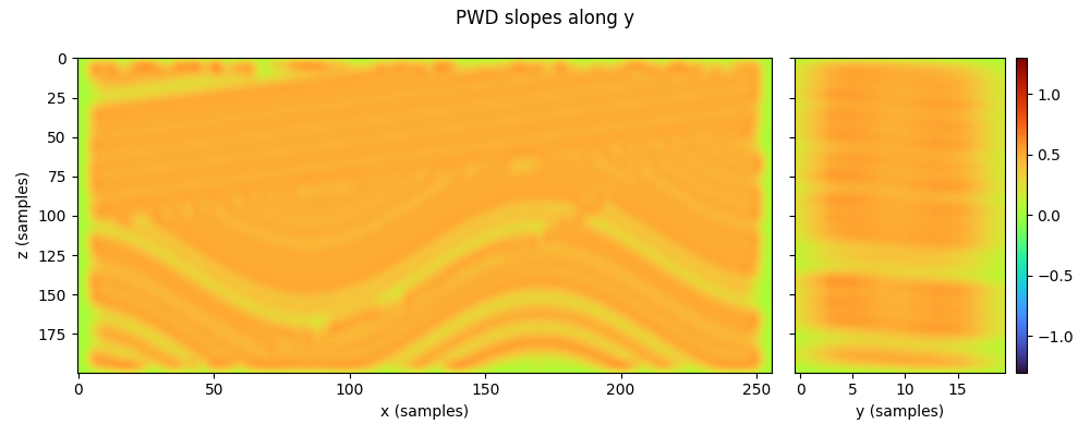
Let’s now compute the PWD slopes along both y and x directions.

pwd_slope3d_y = pwd_slope_estimate(
    sigmoid3d.transpose(1, 2, 0),
    niter=5,
    liter=20,
    order=2,
    nsmooth=(12, 12, 5),
    damp=6e-4,
    smoothing="triangle",
    axis=1,
).transpose(2, 0, 1)

pwd_slope3d_x = pwd_slope_estimate(
    sigmoid3d.transpose(1, 2, 0),
    niter=5,
    liter=20,
    order=2,
    nsmooth=(12, 5, 12),
    damp=6e-4,
    smoothing="triangle",
    axis=2,
).transpose(2, 0, 1)

v = np.max(np.abs(pwd_slope3d_y))

fig, ax = plt.subplots(1, 2, figsize=(10, 4), sharey=True, width_ratios=(3, 1))
fig.suptitle("PWD slopes along x")
ax[0].imshow(pwd_slope3d_y[ny // 2], aspect="auto", cmap="turbo", vmin=-v, vmax=v)
ax[0].set_ylabel("z (samples)")
ax[0].set_xlabel("x (samples)")
im1 = ax[1].imshow(
    pwd_slope3d_y[..., nx // 2].T, aspect="auto", cmap="turbo", vmin=-v, vmax=v
)
ax[1].set_xlabel("y (samples)")
create_colorbar(im1, ax=ax[1])
fig.tight_layout()

fig, ax = plt.subplots(1, 2, figsize=(10, 4), sharey=True, width_ratios=[3, 1])
fig.suptitle("PWD slopes along y")
ax[0].imshow(pwd_slope3d_x[ny // 2], aspect="auto", cmap="turbo", vmin=-v, vmax=v)
ax[0].set_ylabel("z (samples)")
ax[0].set_xlabel("x (samples)")
im1 = ax[1].imshow(
    pwd_slope3d_x[..., nx // 2].T, aspect="auto", cmap="turbo", vmin=-v, vmax=v
)
ax[1].set_xlabel("y (samples)")
create_colorbar(im1, ax=ax[1])
fig.tight_layout()

• 
• 

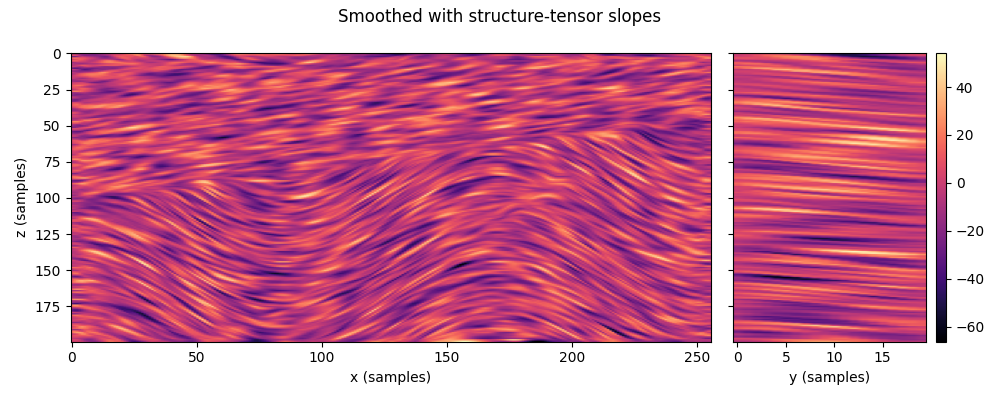
Finally we perform structure-aligned smoothing along both y and x directions.

PWSmoother2D_ = partial(PWSmoother2D, radius=radius, alpha=alpha, dtype="float32")
noise3d = np.random.uniform(-1.0, 1.0, size=(ny, nz, nx)).astype(np.float32)

SOp_pwd3d_y = pylops.BlockDiag(
    [PWSmoother2D_(dims=(nz, nx), sigma=pwd_slope3d_y[i]) for i in range(ny)]
)

SOp_pwd3d_x = pylops.BlockDiag(
    [PWSmoother2D_(dims=(nz, ny), sigma=pwd_slope3d_x[..., i].T) for i in range(nx)]
)
TOp = pylops.Transpose((ny, nz, nx), axes=(2, 1, 0))
SOp_pwd3d_x = TOp.H @ SOp_pwd3d_x @ TOp

SOp_pwd3d = SOp_pwd3d_x @ SOp_pwd3d_y
smooth_st3d = SOp_pwd3d @ noise3d

fig, ax = plt.subplots(1, 2, figsize=(10, 4), sharey=True, width_ratios=(3, 1))
fig.suptitle("Smoothed with structure-tensor slopes")
ax[0].imshow(smooth_st3d[ny // 2], aspect="auto", cmap="magma")
ax[0].set_ylabel("z (samples)")
ax[0].set_xlabel("x (samples)")
im1 = ax[1].imshow(smooth_st3d[..., nx // 2].T, aspect="auto", cmap="magma")
ax[1].set_xlabel("y (samples)")
create_colorbar(im1, ax=ax[1])
fig.tight_layout()