Note

Go to the end to download the full example code.

22. Time-shift estimation¶

This tutorial showcases how one can leverage the extensive suite of PyLops operators to solve nonlinear inverse problems with minimal additional boilerplate code. We will both create a simple nonlinear solver and take advantage of existing solvers provided by third-party library such as SciPy.

We are going to consider a classic problem in signal processing, namely the registration of two signals where one signal is a non-stationary shifted version of the other:

\[d_2(t) = d_1(t - \delta t(t))\]

where $d_1(t)$ and $d_2(t)$ are the two signals to register and $\delta t(t)$ is the time-shift that we want to estimate. When $\delta t(t) > 0$, the second signal is delayed with respect to the first one, whilst when $\delta t(t) < 0$, the second signal is anticipated with respect to the first one.

from functools import partial

import matplotlib.pyplot as plt
import numpy as np
from scipy.optimize import least_squares
from scipy.signal.windows import hamming
from scipy.sparse.linalg import aslinearoperator

import pylops

np.random.seed(10)
plt.close("all")

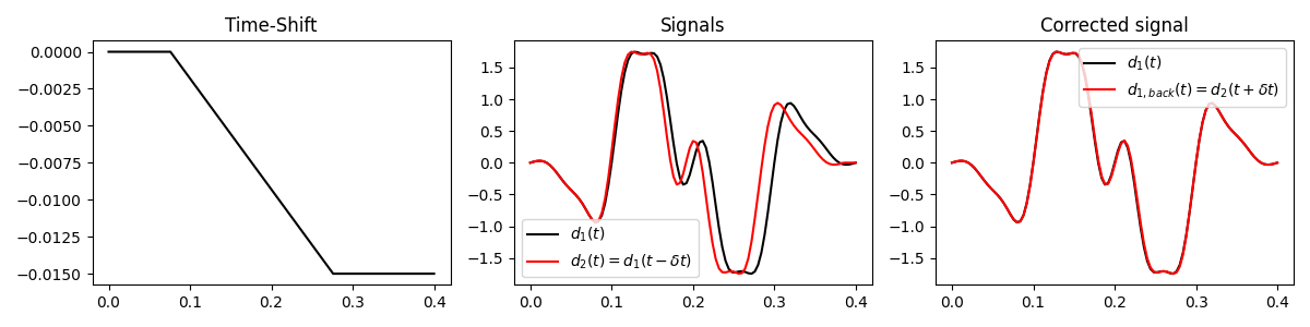
Let’s first create a signal represented by the superposition of three sinusoids and a shifted version of it given a known time-shift function.

# time axis
dt = 0.004
nt = 101
t = np.arange(nt) * dt

# input signal (with taper on the edges)
d1 = (
    np.sin(2 * np.pi * 10 * t)
    + 0.4 * np.sin(2 * np.pi * 20 * t)
    - 2 * np.sin(2 * np.pi * 5 * t)
)
d1 *= hamming(nt)

# define time-shift as integral of a step-like function
steps = np.zeros(nt)
steps[20:70] = -3e-4
shift = np.cumsum(steps)

# apply time-shift
tshift = t - shift
iava = tshift / dt
SOp, iava = pylops.signalprocessing.Interp(nt, iava, kind="sinc")
d2 = SOp @ d1

# revert time-shift
tshift_rev = t + shift
iava_rev = tshift_rev / dt
SOprev, iava_rev = pylops.signalprocessing.Interp(nt, iava_rev, kind="sinc")
d1back = SOprev @ d2

fig, axs = plt.subplots(1, 3, figsize=(12, 3))
axs[0].plot(t, shift, "k")
axs[0].set_title("Time-Shift")

axs[1].plot(t, d1, "k", label=r"$d_1(t)$")
axs[1].plot(t, d2, "r", label=r"$d_2(t)=d_1(t - \delta t)$")
axs[1].legend()
axs[1].set_title("Signals")

axs[2].plot(t, d1, "k", label=r"$d_1(t)$")
axs[2].plot(t, d1back, "r", label=r"$d_{1,back}(t)=d_2(t + \delta t)$")
axs[2].legend()
axs[2].set_title("Corrected signal")
fig.tight_layout()

We can now try to estimate the time-shift function given the two signals by minimizing the following cost function:

\[J(\delta t(t)) = ||d_2(t) - d_1(t - \delta t(t))||^2\]

This is a nonlinear problem as the operator that maps $d_1(t)$ into $d_1(t - \delta t(t))$ depends on the unknown time-shift function $\delta t(t)$. We can however solve this problem iteratively by linearizing the operator around the current estimate of the time-shift function at each iteration. In particular, we can write the Taylor expansion of $d_1(t - \delta t(t))$ around $t$ as:

\[d_1(t - \delta t(t)) = d_1(t) - \frac{\partial d_1}{\partial t}|_t \delta t(t)\]

If we discretize the time axis, we can express this operation in a matrix-vector:

\[\mathbf{d}_{1, \boldsymbol \delta_\mathbf{t}} = \mathbf{d}_1 + \mathbf{J} \boldsymbol \delta \mathbf{t}\]

where the Jacobian matrix is given by $\mathbf{J}= -diag\{\frac{\partial \mathbf{d}_1}{\partial t}|_{t=t}\}$.

We can now solve the following linear least-squares problem:

\[J = ||(\mathbf{d}_2 - \mathbf{d}_1) - \mathbf{J} \boldsymbol \delta \mathbf{t})||_2^2 + \epsilon ||\nabla \boldsymbol \delta \mathbf{t}||_2^2\]

where a regularization term is added to promote smooth solutions.

# data term
ddiff = d2 - d1

# Jacobian
DOp = pylops.FirstDerivative(nt, sampling=dt, edge=True)
J = -pylops.Diagonal(DOp @ d1)

# second derivative regularization
D2Op = pylops.SecondDerivative(nt)

# inversion
shift_est = pylops.optimization.leastsquares.regularized_inversion(
    J,
    ddiff,
    [
        D2Op,
    ],
    epsRs=[
        1e3,
    ],
    **dict(iter_lim=200)
)[0]

# revert time-shift (with estimated shift)
tshift_est = t + shift_est
iava_est = tshift_est / dt
SOpest, iava_est = pylops.signalprocessing.Interp(nt, iava_est, kind="sinc")
d1back_est = SOpest * d2

fig, axs = plt.subplots(1, 2, figsize=(12, 3))
axs[0].plot(t, shift, "k", label="True")
axs[0].plot(t, shift_est, "r", label="Estimated")
axs[0].set_title("Shifts")

axs[1].plot(t, d1, "k", label=r"$d_1(t)$")
axs[1].plot(t, d1back_est, "r", label=r"$d_{1,back}(t)=d_2(t + \delta \tilde{t})$")
axs[1].plot(t, d1 - d1back_est, "k", lw=0.5)
axs[1].legend()
axs[1].set_title("Corrected signal")
fig.tight_layout()

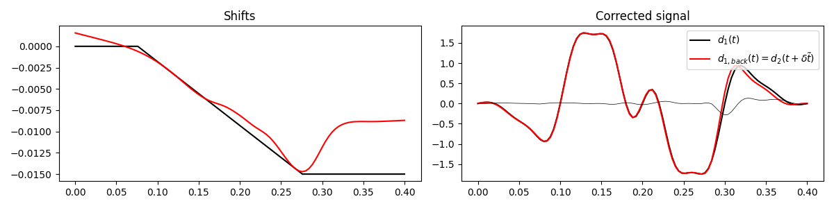
We can see that the estimated time-shift closely matches the true one and that the corrected signal is very similar to the original one. However, we have so far discarded the higher order terms in the Taylor expansion of $d_1(t - \delta t(t))$. We can therefore try to improve our estimate by iterating the above procedure a few times, updating the Jacobian at each iteration with the current estimate of the time-shift function. In other words, at each iteration $i=0,1,...$, we perform the following steps:

Compute the Jacobian $\mathbf{J}^{i}= -diag\{\frac{\partial \tilde{\mathbf{d}}^i_1}{\partial t}|_{t=t}\}$
Solve the linear least-squares problem

\[J = ||(\mathbf{d}_2 - \tilde{\mathbf{d}}^i_1) - \mathbf{J}^i \boldsymbol \Delta \mathbf{t}^{i+1})||_2^2 + \epsilon ||\nabla (\boldsymbol \Delta \mathbf{t}^{i+1} + \boldsymbol \delta \mathbf{t}^i)||_2^2\]
Update the time-shift estimate as $\delta t^{i+1}(t) = \delta t^i(t) + \Delta t^{i+1}(t)$ We can repeat these steps until convergence is reached.
Time shift $d_1^{i+1}(t)$ with the current estimate of the time-shift function: $\tilde{d}_1^{i+1}(t) = d_1^i(t + \delta t^{i+1}(t))$

with $\delta t^0(t)=0$ and $\tilde{d}_1^0(t)=d_1(t)$.

# number of outer iterations
niter = 10

# pre-compute derivative operators
Dop = pylops.FirstDerivative(nt, edge=True)
D2Op = pylops.SecondDerivative(nt)

shift_estgn = np.zeros(nt)
shift_estgn_hist = np.zeros((niter, nt))

d1shift = d1.copy()
Jhist_gn = []

for iiter in range(niter):

    # data term
    ddiff = d2 - d1shift

    # compute residual norm
    Jhist_gn.append(np.linalg.norm(ddiff))

    # Jacobian
    J = -pylops.Diagonal((Dop @ d1shift) / dt)

    # inversion
    shift_estgn += pylops.optimization.leastsquares.regularized_inversion(
        J,
        ddiff,
        [
            D2Op,
        ],
        epsRs=[
            5e2,
        ],
        dataregs=[
            -D2Op * shift_estgn,
        ],
        **dict(iter_lim=100, damp=1e-4)
    )[0]
    shift_estgn_hist[iiter] = shift_estgn

    # revert current time-shift estimate
    iava_gn = (t - shift_estgn) / dt
    SOpgn, _ = pylops.signalprocessing.Interp(nt, iava_gn, kind="sinc")
    d1shift = SOpgn @ d1

# compute final residual norm
Jhist_gn.append(np.linalg.norm(d2 - d1shift))

# revert time-shift (with estimated shift)
tshift_est = t + shift_estgn
iava_est = tshift_est / dt
SOpest, iava_est = pylops.signalprocessing.Interp(nt, iava_est, kind="sinc")
d1back_estgn = SOpest * d2

fig, axs = plt.subplots(1, 3, figsize=(12, 3))
axs[0].plot(t, shift, "k", lw=2, label="True")
axs[0].plot(t, shift_estgn, "r", lw=2, label="Estimated")
axs[0].plot(t, shift_estgn_hist.T, "r", lw=0.5, alpha=0.4)
axs[0].set_title("Shifts")

axs[1].plot(t, d1, "k", label=r"$d_1(t)$")
axs[1].plot(t, d1back_estgn, "r", label=r"$d_{1,back}(t)=d_2(t + \delta \tilde{t})$")
axs[1].plot(t, d1 - d1back_estgn, "k", lw=0.5)
axs[1].legend()
axs[1].set_title("Corrected signal")

axs[2].plot(Jhist_gn, "k")
axs[2].set_title("Residual Norm")
fig.tight_layout()

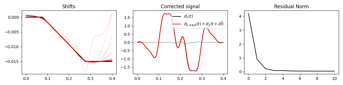
A much better match! However, since we have alternated here the solution of linearized systems of equations (for an update in the time-shift) with a partial shifting of the input signal $d_1(t)$ with the current estimate of the time-shift, this pattern makes our solver very be-spoke.

Next, we will see that if we sligthly reformulate our problem in such a way that partial shifting is not required, we can take advantage of an existing solver provided by a third-party library such as SciPy. To begin with, let’s rewrite a generic Taylor expansion for $d_1(t - \delta t^{i+1}(t))$ around $\delta t^i(t)$:

\[d_1(t - \delta t^{i+1}(t)) = d_1((t - \delta t^i(t)) - \Delta t^{i+1}(t)) = d_1(t) - \frac{\partial d_1}{\partial t} |_{t=t-\delta t^i(t)} \Delta t^{i+1}(t)\]

Again, if we discretize the time axis, we can express this operation in a matrix-vector:

\[\mathbf{d}_{1, \boldsymbol \delta_\mathbf{t}^{i+1}} = \mathbf{d}^i_1 + \mathbf{J}^i \boldsymbol \Delta \mathbf{t}^{i+1}\]

where the Jacobian matrix is given by $\mathbf{J}^i= -diag\{\frac{\partial \mathbf{d}_1}{\partial t}|_{t=t-\delta t^i(t)}\}$.

By doing so, we can now solve a series of linearized problems of the form:

\[J^{i+1} = ||(\mathbf{d}_2 - \tilde{\mathbf{d}}^i_1) - \mathbf{J}^i \boldsymbol \Delta \mathbf{t}^{i+1})||_2^2 + \epsilon ||\nabla (\boldsymbol \Delta \mathbf{t}^{i+1} + \boldsymbol \delta \mathbf{t}^i)||_2^2\]

where $\tilde{d}_1^i(t) = d_1^i(t + \delta t^i(t))$, $\delta t^0(t)=0$, and $\tilde{d}_1^0(t)=d_1(t)$. This series of problems now amenable to the scipy.optimize.least_squares method. In practice, all we need to be able to create is two methods: the first, called fun, must return the inner part of the objective function, the latter, called jacobian must create a linear operator that acts like the Jacobian of the augmented system.

def fun(x, d1, d2, t, dt, eps):
    nt = len(t)
    iava = (t - x) / dt
    SOpest, iava = pylops.signalprocessing.Interp(nt, iava, kind="sinc")
    D2Op = pylops.SecondDerivative(nt)

    d1shift = SOpest * d1
    res = d2 - d1shift
    resr = D2Op * x
    return np.hstack((res, eps * resr))


def jacobian(x, d1, d2, t, dt, eps):
    nt = len(t)
    iava = (t - x) / dt
    SOpest, _ = pylops.signalprocessing.Interp(nt, iava, kind="sinc")
    S1Opest, _ = pylops.signalprocessing.Interp(nt, iava + 1, kind="sinc")
    J = (S1Opest * d1 - SOpest * d1) / dt
    D2Op = pylops.SecondDerivative(nt)
    J = pylops.VStack([pylops.Diagonal(J), eps * D2Op])
    J = aslinearoperator(J)
    return J


def callback(x, t, dt, d1, d2):
    iava = (t - x) / dt
    SOpgn, _ = pylops.signalprocessing.Interp(nt, iava, kind="sinc")
    d1shift = SOpgn @ d1
    shift_estls_hist.append(x)
    Jhist_ls.append(np.linalg.norm(d2 - d1shift))


eps = 8e1
shift_estls_hist = []
Jhist_ls = []
shift_estls = least_squares(
    fun,
    np.zeros(nt),
    jac=jacobian,
    method="trf",
    verbose=1,
    args=(d1, d2, t, dt, eps),
    callback=partial(callback, t=t, dt=dt, d1=d1, d2=d2),
).x

# revert time-shift (with estimated shift)
tshift_estls = t + shift_estls
iava_estls = tshift_estls / dt
SOpestls, iava_estls = pylops.signalprocessing.Interp(nt, iava_estls, kind="sinc")
d1back_estls = SOpestls * d2

fig, axs = plt.subplots(1, 3, figsize=(12, 3))
axs[0].plot(t, shift, "k", lw=2, label="True")
axs[0].plot(t, shift_estls, "r", lw=2, label="Estimated")
axs[0].plot(t, np.vstack(shift_estls_hist).T, "r", lw=0.5, alpha=0.4)
axs[0].set_title("Shifts")

axs[1].plot(t, d1, "k", label=r"$d_1(t)$")
axs[1].plot(t, d1back_estls, "r", label=r"$d_{1,back}(t)=d_2(t + \delta \tilde{t})$")
axs[1].plot(t, d1 - d1back_estls, "k", lw=0.5)
axs[1].legend()
axs[1].set_title("Corrected signal")

axs[2].plot(Jhist_ls, "k")
axs[2].set_title("Residual Norm")
fig.tight_layout()

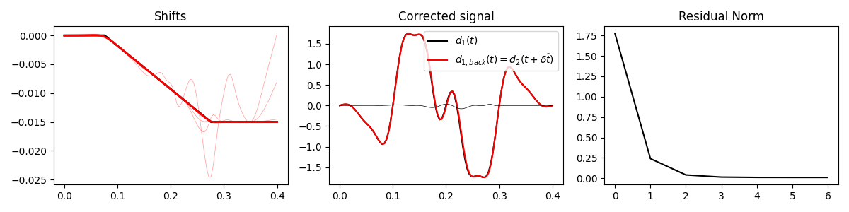
`xtol` termination condition is satisfied.
Function evaluations 15, initial cost 8.8169e+00, final cost 1.5930e-04, first-order optimality 1.17e-02.

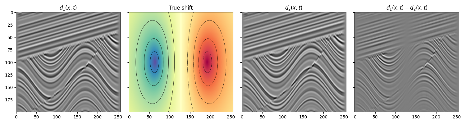
Finally, we repeat the same exercise with a 2-dimensional dataset. Here, each trace is time shifted independently, however a pylops.Laplacian operator is used to ensure smoothness in the solution across traces.

Let’s start by loading a 2D dataset

inputfile = "../testdata/sigmoid.npz"

d1 = 1e3 * np.load(inputfile)["sigmoid"]
nx, nz = d1.shape
x = np.linspace(-500.0, 500.0, nx)
z = np.linspace(0.0, 400.0, nz)
X, Z = np.meshgrid(x, z, indexing="ij")

Next, we define a shift composed of two gaussians with opposite polarity on either side of the x-axis

dt = 0.004
t = np.arange(nz) * dt
shift = np.exp(-np.sqrt((X + 250) ** 2 + (Z - 200) ** 2) / 200) - np.exp(
    -np.sqrt((X - 250) ** 2 + (Z - 200) ** 2) / 200
)
shift = 4e-4 * shift / shift.max()

# apply time-shift
tshift = t[np.newaxis, :] - shift
iavas = tshift / dt
SOp = pylops.BlockDiag(
    [pylops.signalprocessing.Interp(nz, iava, kind="sinc")[0] for iava in iavas]
)
d2 = SOp * d1

# revert time-shift
tshift_rev = t[np.newaxis, :] + shift
iavas_rev = tshift_rev / dt
SOprev = pylops.BlockDiag(
    [pylops.signalprocessing.Interp(nz, iava, kind="sinc")[0] for iava in iavas_rev]
)
d2shifted = SOprev * d2

v = np.max(np.abs(shift))
fig, axs = plt.subplots(1, 4, figsize=(15, 4), sharey=True)
axs[0].imshow(d1.T, aspect="auto", cmap="gray")
axs[0].set_title(r"$d_1(x, t)$")
axs[1].imshow(shift.T, aspect="auto", cmap="Spectral", vmin=-v, vmax=v)
axs[1].contour(shift.T, levels=np.linspace(-4e-4, 4e-4, 11), colors="k", linewidths=0.5)
axs[1].set_title("True shift")
axs[2].imshow(d2.T, aspect="auto", cmap="gray")
axs[2].set_title(r"$d_2(x, t)$")
axs[3].imshow(d1.T - d2.T, aspect="auto", cmap="gray")
axs[3].set_title(r"$d_1(x, t) - d_2(x, t)$")
fig.tight_layout()

$d_1(x, t)$, True shift, $d_2(x, t)$, $d_1(x, t) - d_2(x, t)$

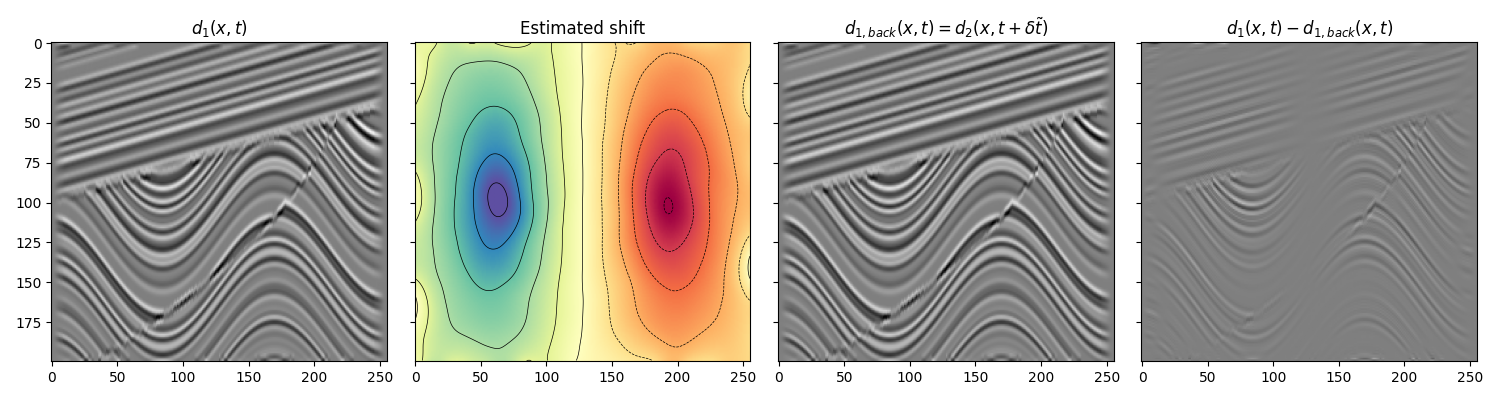
Like in the 1D, we start with a single linearization

# data term
ddiff = d2 - d1

# Jabobian
DOp = pylops.FirstDerivative((nx, nz), axis=-1, sampling=dt, edge=True)
J = -pylops.Diagonal(DOp @ d1)

# laplacian regularization
D2Op = pylops.Laplacian(dims=(nx, nz))

shift_est = pylops.optimization.leastsquares.regularized_inversion(
    J,
    ddiff.ravel(),
    [
        D2Op,
    ],
    epsRs=[
        1e4,
    ],
    **dict(iter_lim=1000)
)[0]
shift_est = shift_est.reshape(nx, nz)

# shift back
tshift_est = t[np.newaxis, :] + shift_est
iavas_est = tshift_est / dt
SOpest = pylops.BlockDiag(
    [pylops.signalprocessing.Interp(nz, iava, kind="sinc")[0] for iava in iavas_est]
)
d1back_est = SOpest * d2

fig, axs = plt.subplots(1, 4, figsize=(15, 4), sharey=True)
axs[0].imshow(d1.T, aspect="auto", cmap="gray", vmin=-5.0, vmax=5.0)
axs[0].set_title(r"$d_1(x, t)$")
axs[1].imshow(shift_est.T, aspect="auto", cmap="Spectral", vmin=-v, vmax=v)
axs[1].contour(
    shift_est.T, levels=np.linspace(-4e-4, 4e-4, 11), colors="k", linewidths=0.5
)
axs[1].set_title("Estimated shift")
axs[2].imshow(d1back_est.T, aspect="auto", cmap="gray", vmin=-5.0, vmax=5.0)
axs[2].set_title(r"$d_{1,back}(x, t)=d_2(x, t + \delta \tilde{t})$")
axs[3].imshow(d1.T - d1back_est.T, aspect="auto", cmap="gray", vmin=-0.1, vmax=0.1)
axs[3].set_title(r"$d_1(x, t) - d_{1,back}(x, t)$")
fig.tight_layout()

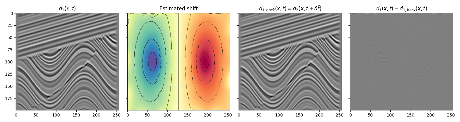
$d_1(x, t)$, Estimated shift, $d_{1,back}(x, t)=d_2(x, t + \delta \tilde{t})$, $d_1(x, t) - d_{1,back}(x, t)$

And finally by a series of linearizations using scipy.optimize.least_squares

def fun(x, d1, d2, t, dt, eps):
    nt = len(t)
    nx = x.size // nt
    iavas = (t[np.newaxis, :] - x.reshape(nx, nt)) / dt
    SOpest = pylops.BlockDiag(
        [pylops.signalprocessing.Interp(nt, iava, kind="sinc")[0] for iava in iavas]
    )
    D2Op = pylops.Laplacian((nx, nt))

    d1shift = SOpest * d1.ravel()
    res = d2.ravel() - d1shift
    resr = D2Op * x
    return np.hstack((res, eps * resr))


def jacobian(x, d1, d2, t, dt, eps):
    nt = len(t)
    nx = x.size // nt
    iavas = (t[np.newaxis, :] - x.reshape(nx, nt)) / dt
    SOpest = pylops.BlockDiag(
        [pylops.signalprocessing.Interp(nt, iava, kind="sinc")[0] for iava in iavas]
    )
    S1Opest = pylops.BlockDiag(
        [pylops.signalprocessing.Interp(nt, iava + 1, kind="sinc")[0] for iava in iavas]
    )
    J = (S1Opest * d1.ravel() - SOpest * d1.ravel()) / dt
    D2Op = pylops.Laplacian((nx, nt))
    J = pylops.VStack([pylops.Diagonal(J), eps * D2Op])
    J = aslinearoperator(J)
    return J


def callback(x, t, dt, d1, d2):
    nt = len(t)
    nx = x.size // nt
    iavas = (t[np.newaxis, :] - x.reshape(nx, nt)) / dt
    SOpgn = pylops.BlockDiag(
        [pylops.signalprocessing.Interp(nt, iava, kind="sinc")[0] for iava in iavas]
    )
    d1shift = SOpgn @ d1.ravel()
    shift_estls_hist.append(x)
    Jhist_ls.append(np.linalg.norm(d2.ravel() - d1shift))


eps = 5e2
shift_estls_hist = []
Jhist_ls = []
shift_estls = least_squares(
    fun,
    np.zeros(nx * nz),
    jac=jacobian,
    method="trf",
    verbose=1,
    args=(d1, d2, t, dt, eps),
    callback=partial(callback, t=t, dt=dt, d1=d1, d2=d2),
).x

shift_estls = shift_estls.reshape(nx, nz)

# revert time-shift
tshift_estls = t[np.newaxis, :] + shift_estls
iavas_estls = tshift_estls / dt
SOpestls = pylops.BlockDiag(
    [pylops.signalprocessing.Interp(nz, iava, kind="sinc")[0] for iava in iavas_estls]
)
d1back_estls = SOpestls * d2

fig, axs = plt.subplots(1, 4, figsize=(15, 4), sharey=True)
axs[0].imshow(d1.T, aspect="auto", cmap="gray", vmin=-5.0, vmax=5.0)
axs[0].set_title(r"$d_1(x, t)$")
axs[1].imshow(shift_est.T, aspect="auto", cmap="Spectral", vmin=-v, vmax=v)
axs[1].contour(
    shift_estls.T, levels=np.linspace(-4e-4, 4e-4, 11), colors="k", linewidths=0.5
)
axs[1].set_title("Estimated shift")
axs[2].imshow(d1back_estls.T, aspect="auto", cmap="gray", vmin=-5.0, vmax=5.0)
axs[2].set_title(r"$d_{1,back}(x, t)=d_2(x, t + \delta \tilde{t})$")
axs[3].imshow(d1.T - d1back_estls.T, aspect="auto", cmap="gray", vmin=-0.1, vmax=0.1)
axs[3].set_title(r"$d_1(x, t) - d_{1,back}(x, t)$")
fig.tight_layout()

fig, axs = plt.subplots(1, 2, figsize=(15, 4))

axs[0].plot(t, shift[nx // 4], "k", label="True")
axs[0].plot(t, shift_est[nx // 4], "r", label="Linearized")
axs[0].plot(t, shift_estls[nx // 4], "b", label="LS")
axs[0].plot(t, shift[-nx // 4], "k")
axs[0].plot(t, shift_est[-nx // 4], "r")
axs[0].plot(t, shift_estls[-nx // 4], "b")
axs[0].set_title("Shifts")
axs[0].legend()

axs[1].plot(Jhist_ls, "k")
axs[1].set_title("Residual Norm")
fig.tight_layout()

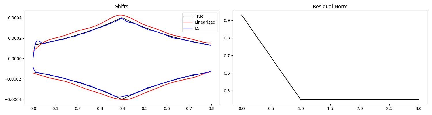
$d_1(x, t)$, Estimated shift, $d_{1,back}(x, t)=d_2(x, t + \delta \tilde{t})$, $d_1(x, t) - d_{1,back}(x, t)$

`xtol` termination condition is satisfied.
Function evaluations 15, initial cost 5.5323e+01, final cost 1.2254e-01, first-order optimality 5.18e+01.

Total running time of the script: (0 minutes 12.660 seconds)

Gallery generated by Sphinx-Gallery