Operators concatenation

This example shows how to use ‘stacking’ operators such as pylops.VStack, pylops.HStack, pylops.Block, pylops.BlockDiag, and pylops.Kronecker.

These operators allow for different combinations of multiple linear operators in a single operator. Such functionalities are used within PyLops as the basis for the creation of complex operators as well as in the definition of various types of optimization problems with regularization or preconditioning.

Some of this operators naturally lend to embarassingly parallel computations. Within PyLops we leverage the Multiprocessing module to run multiple processes at the same time evaluating a subset of the operators involved in one of the stacking operations.

import matplotlib.pyplot as plt
import numpy as np

import pylops

plt.close("all")

Let’s start by defining two second derivatives pylops.SecondDerivative that we will be using in this example.

D2hop = pylops.SecondDerivative(dims=(11, 21), axis=1, dtype="float32")
D2vop = pylops.SecondDerivative(dims=(11, 21), axis=0, dtype="float32")

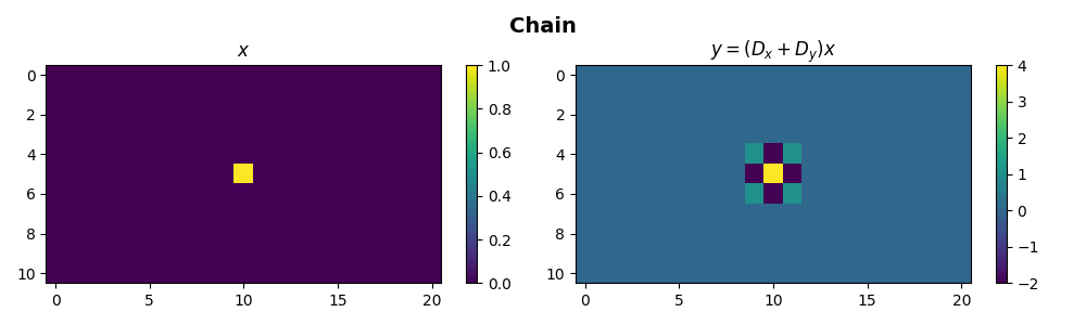
Chaining of operators represents the simplest concatenation that can be performed between two or more linear operators. This can be easily achieved using the * symbol

\[\mathbf{D_{cat}}= \mathbf{D_v} \mathbf{D_h}\]

Nv, Nh = 11, 21
X = np.zeros((Nv, Nh))
X[int(Nv / 2), int(Nh / 2)] = 1

D2op = D2vop * D2hop
Y = D2op * X

fig, axs = plt.subplots(1, 2, figsize=(10, 3))
fig.suptitle("Chain", fontsize=14, fontweight="bold", y=0.95)
im = axs[0].imshow(X, interpolation="nearest")
axs[0].axis("tight")
axs[0].set_title(r"$x$")
plt.colorbar(im, ax=axs[0])
im = axs[1].imshow(Y, interpolation="nearest")
axs[1].axis("tight")
axs[1].set_title(r"$y=(D_x+D_y) x$")
plt.colorbar(im, ax=axs[1])
plt.tight_layout()
plt.subplots_adjust(top=0.8)

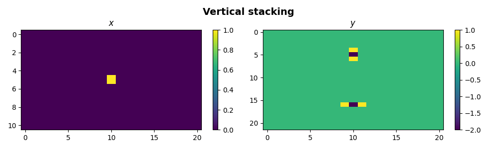
We now want to vertically stack three operators

\[\begin{split}\mathbf{D_{Vstack}} = \begin{bmatrix} \mathbf{D_v} \\ \mathbf{D_h} \end{bmatrix}, \qquad \mathbf{y} = \begin{bmatrix} \mathbf{D_v}\mathbf{x} \\ \mathbf{D_h}\mathbf{x} \end{bmatrix}\end{split}\]

Nv, Nh = 11, 21
X = np.zeros((Nv, Nh))
X[int(Nv / 2), int(Nh / 2)] = 1
Dstack = pylops.VStack([D2vop, D2hop])

Y = np.reshape(Dstack * X.ravel(), (Nv * 2, Nh))

fig, axs = plt.subplots(1, 2, figsize=(10, 3))
fig.suptitle("Vertical stacking", fontsize=14, fontweight="bold", y=0.95)
im = axs[0].imshow(X, interpolation="nearest")
axs[0].axis("tight")
axs[0].set_title(r"$x$")
plt.colorbar(im, ax=axs[0])
im = axs[1].imshow(Y, interpolation="nearest")
axs[1].axis("tight")
axs[1].set_title(r"$y$")
plt.colorbar(im, ax=axs[1])
plt.tight_layout()
plt.subplots_adjust(top=0.8)

If one now wants to have one or more null operators in the stack, it is reccomended to use the pylops.Zero operator (instead of, for example, a pylops.MatrixMult filled with a zero matrix); under the hood, a pylops.Zero operator will be simply by-passed both in the forward and adjoint steps.

\[\begin{split}\mathbf{D_{Vstack}} = \begin{bmatrix} \mathbf{D_v} \\ \mathbf{0} \\ \mathbf{D_h} \end{bmatrix}, \qquad \mathbf{y} = \begin{bmatrix} \mathbf{D_v}\mathbf{x} \\ \mathbf{0} \\ \mathbf{D_h}\mathbf{x} \end{bmatrix}\end{split}\]

Note that this feature will become particularly handy when defining pylops.Block operators with large zero blocks.

# With MatrixMult operator filled with zeros
Zop = pylops.MatrixMult(np.zeros((Nv * Nh, Nv * Nh)))
Dstack = pylops.VStack([D2vop, Zop, D2hop])
Y = np.reshape(Dstack * X.ravel(), (Nv * 3, Nh))

# With Zero operator
Zop = pylops.Zero(Nv * Nh)
D1stack = pylops.VStack([D2vop, Zop, D2hop])
Y1 = np.reshape(D1stack * X.ravel(), (Nv * 3, Nh))

print("Y == Y1:", np.allclose(Y, Y1))

Y == Y1: True

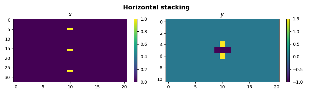
Similarly we can now horizontally stack three operators

\[\mathbf{D_{Hstack}} = \begin{bmatrix} \mathbf{D_v} & 0.5*\mathbf{D_v} & -1*\mathbf{D_h} \end{bmatrix}, \qquad \mathbf{y} = \mathbf{D_v}\mathbf{x}_1 + 0.5*\mathbf{D_v}\mathbf{x}_2 - \mathbf{D_h}\mathbf{x}_3\]

Nv, Nh = 11, 21
X = np.zeros((Nv * 3, Nh))
X[int(Nv / 2), int(Nh / 2)] = 1
X[int(Nv / 2) + Nv, int(Nh / 2)] = 1
X[int(Nv / 2) + 2 * Nv, int(Nh / 2)] = 1

Hstackop = pylops.HStack([D2vop, 0.5 * D2vop, -1 * D2hop])
Y = np.reshape(Hstackop * X.ravel(), (Nv, Nh))

fig, axs = plt.subplots(1, 2, figsize=(10, 3))
fig.suptitle("Horizontal stacking", fontsize=14, fontweight="bold", y=0.95)
im = axs[0].imshow(X, interpolation="nearest")
axs[0].axis("tight")
axs[0].set_title(r"$x$")
plt.colorbar(im, ax=axs[0])
im = axs[1].imshow(Y, interpolation="nearest")
axs[1].axis("tight")
axs[1].set_title(r"$y$")
plt.colorbar(im, ax=axs[1])
plt.tight_layout()
plt.subplots_adjust(top=0.8)

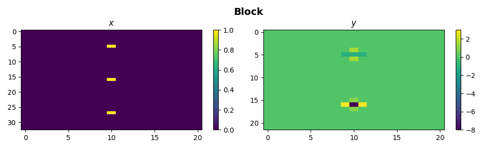
We can even stack them both horizontally and vertically such that we create a block operator

\[\begin{split}\mathbf{D_{Block}} = \begin{bmatrix} \mathbf{D_v} & 0.5*\mathbf{D_v} & -1*\mathbf{D_h} \\ \mathbf{D_h} & 2*\mathbf{D_h} & \mathbf{D_v} \\ \end{bmatrix}, \qquad \mathbf{y} = \begin{bmatrix} \mathbf{D_v} \mathbf{x_1} + 0.5*\mathbf{D_v} \mathbf{x_2} - \mathbf{D_h} \mathbf{x_3} \\ \mathbf{D_h} \mathbf{x_1} + 2*\mathbf{D_h} \mathbf{x_2} + \mathbf{D_v} \mathbf{x_3} \end{bmatrix}\end{split}\]

Bop = pylops.Block([[D2vop, 0.5 * D2vop, -1 * D2hop], [D2hop, 2 * D2hop, D2vop]])
Y = np.reshape(Bop * X.ravel(), (2 * Nv, Nh))

fig, axs = plt.subplots(1, 2, figsize=(10, 3))
fig.suptitle("Block", fontsize=14, fontweight="bold", y=0.95)
im = axs[0].imshow(X, interpolation="nearest")
axs[0].axis("tight")
axs[0].set_title(r"$x$")
plt.colorbar(im, ax=axs[0])
im = axs[1].imshow(Y, interpolation="nearest")
axs[1].axis("tight")
axs[1].set_title(r"$y$")
plt.colorbar(im, ax=axs[1])
plt.tight_layout()
plt.subplots_adjust(top=0.8)

And here with some Zero blocks

\[\begin{split}\mathbf{D_{Block}} = \begin{bmatrix} \mathbf{D_v} & \mathbf{0} & -1*\mathbf{D_h} \\ \mathbf{D_h} & 2*\mathbf{D_h} & \mathbf{0} \\ \end{bmatrix}, \qquad \mathbf{y} = \begin{bmatrix} \mathbf{D_v} \mathbf{x_1} - \mathbf{D_h} \mathbf{x_3} \\ \mathbf{D_h} \mathbf{x_1} + 2*\mathbf{D_h} \mathbf{x_2} \end{bmatrix}\end{split}\]

# With MatrixMult operator filled with zeros
Zop = pylops.MatrixMult(np.zeros(D2vop.shape))
Bop = pylops.Block([[D2vop, Zop, -1 * D2hop], [D2hop, 2 * D2hop, Zop]])
Y = np.reshape(Bop * X.ravel(), (2 * Nv, Nh))

# With Zero operator
Zop = pylops.Zero(D2vop.shape[0])
B1op = pylops.Block([[D2vop, Zop, -1 * D2hop], [D2hop, 2 * D2hop, Zop]])
Y1 = np.reshape(B1op * X.ravel(), (2 * Nv, Nh))

print("Y == Y1:", np.allclose(Y, Y1))

Y == Y1: True

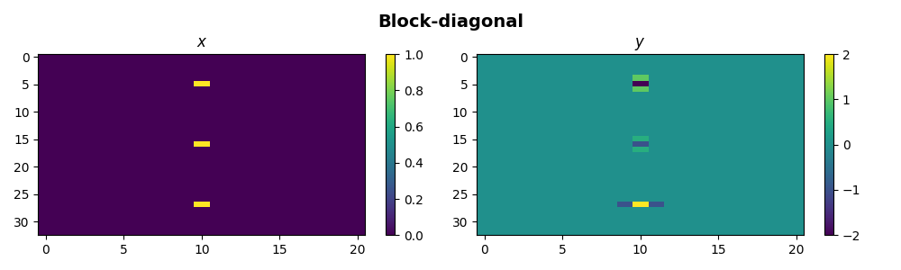
Finally we can use the block-diagonal operator to apply three operators to three different subset of the model and data

\[\begin{split}\mathbf{D_{BDiag}} = \begin{bmatrix} \mathbf{D_v} & \mathbf{0} & \mathbf{0} \\ \mathbf{0} & 0.5*\mathbf{D_v} & \mathbf{0} \\ \mathbf{0} & \mathbf{0} & -\mathbf{D_h} \end{bmatrix}, \qquad \mathbf{y} = \begin{bmatrix} \mathbf{D_v} \mathbf{x_1} \\ 0.5*\mathbf{D_v} \mathbf{x_2} \\ -\mathbf{D_h} \mathbf{x_3} \end{bmatrix}\end{split}\]

BD = pylops.BlockDiag([D2vop, 0.5 * D2vop, -1 * D2hop])
Y = np.reshape(BD * X.ravel(), (3 * Nv, Nh))

fig, axs = plt.subplots(1, 2, figsize=(10, 3))
fig.suptitle("Block-diagonal", fontsize=14, fontweight="bold", y=0.95)
im = axs[0].imshow(X, interpolation="nearest")
axs[0].axis("tight")
axs[0].set_title(r"$x$")
plt.colorbar(im, ax=axs[0])
im = axs[1].imshow(Y, interpolation="nearest")
axs[1].axis("tight")
axs[1].set_title(r"$y$")
plt.colorbar(im, ax=axs[1])
plt.tight_layout()
plt.subplots_adjust(top=0.8)

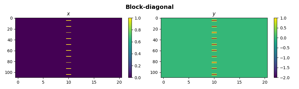
If we consider now the case of having a large number of operators inside a blockdiagonal structure, it may be convenient to span multiple processes handling subset of operators at the same time. This can be easily achieved by simply defining the number of processes we want to use via nproc.

X = np.zeros((Nv * 10, Nh))
for iv in range(10):
    X[int(Nv / 2) + iv * Nv, int(Nh / 2)] = 1

BD = pylops.BlockDiag([D2vop] * 10, nproc=2)
print("BD Operator multiprocessing pool", BD.pool)
Y = np.reshape(BD * X.ravel(), (10 * Nv, Nh))
BD.pool.close()

fig, axs = plt.subplots(1, 2, figsize=(10, 3))
fig.suptitle("Block-diagonal", fontsize=14, fontweight="bold", y=0.95)
im = axs[0].imshow(X, interpolation="nearest")
axs[0].axis("tight")
axs[0].set_title(r"$x$")
plt.colorbar(im, ax=axs[0])
im = axs[1].imshow(Y, interpolation="nearest")
axs[1].axis("tight")
axs[1].set_title(r"$y$")
plt.colorbar(im, ax=axs[1])
plt.tight_layout()
plt.subplots_adjust(top=0.8)

BD Operator multiprocessing pool <multiprocessing.pool.Pool state=RUN pool_size=2>

Finally we use the Kronecker operator and replicate this example on wiki.

\[\begin{split}\begin{bmatrix} 1 & 2 \\ 3 & 4 \\ \end{bmatrix} \otimes \begin{bmatrix} 0 & 5 \\ 6 & 7 \\ \end{bmatrix} = \begin{bmatrix} 0 & 5 & 0 & 10 \\ 6 & 7 & 12 & 14 \\ 0 & 15 & 0 & 20 \\ 18 & 21 & 24 & 28 \\ \end{bmatrix}\end{split}\]

A = np.array([[1, 2], [3, 4]])
B = np.array([[0, 5], [6, 7]])
AB = np.kron(A, B)

n1, m1 = A.shape
n2, m2 = B.shape

Aop = pylops.MatrixMult(A)
Bop = pylops.MatrixMult(B)

ABop = pylops.Kronecker(Aop, Bop)
x = np.ones(m1 * m2)

y = AB.dot(x)
yop = ABop * x
xinv = ABop / yop

print(f"AB = \n {AB}")

print(f"x = {x}")
print(f"y = {y}")
print(f"yop = {yop}")
print(f"xinv = {xinv}")

AB =
 [[ 0  5  0 10]
 [ 6  7 12 14]
 [ 0 15  0 20]
 [18 21 24 28]]
x = [1. 1. 1. 1.]
y = [15. 39. 35. 91.]
yop = [15. 39. 35. 91.]
xinv = [1. 1. 1. 1.]

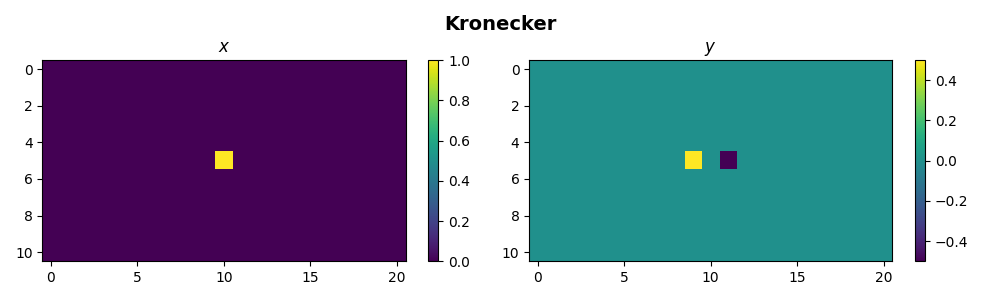
We can also use pylops.Kronecker to do something more interesting. Any operator can in fact be applied on a single direction of a multi-dimensional input array if combined with an pylops.Identity operator via Kronecker product. We apply here the pylops.FirstDerivative to the second dimension of the model.

Note that for those operators whose implementation allows their application to a single axis via the axis parameter, using the Kronecker product would lead to slower performance. Nevertheless, the Kronecker product allows any other operator to be applied to a single dimension.

Nv, Nh = 11, 21

Iop = pylops.Identity(Nv, dtype="float32")
D2hop = pylops.FirstDerivative(Nh, dtype="float32")

X = np.zeros((Nv, Nh))
X[Nv // 2, Nh // 2] = 1
D2hop = pylops.Kronecker(Iop, D2hop)

Y = D2hop * X.ravel()
Y = Y.reshape(Nv, Nh)

fig, axs = plt.subplots(1, 2, figsize=(10, 3))
fig.suptitle("Kronecker", fontsize=14, fontweight="bold", y=0.95)
im = axs[0].imshow(X, interpolation="nearest")
axs[0].axis("tight")
axs[0].set_title(r"$x$")
plt.colorbar(im, ax=axs[0])
im = axs[1].imshow(Y, interpolation="nearest")
axs[1].axis("tight")
axs[1].set_title(r"$y$")
plt.colorbar(im, ax=axs[1])
plt.tight_layout()
plt.subplots_adjust(top=0.8)