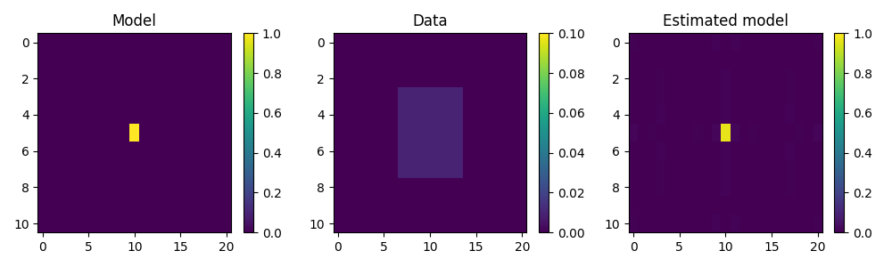
3D Smoothing

This example shows how to use the pylops.SmoothingND operator to smooth a three-dimensional input signal along all axes.

import matplotlib.pyplot as plt
import numpy as np

import pylops

plt.close("all")

Define the input parameters: number of samples of input signal (N1, N2, and N3) and lenght of the smoothing filter regression coefficients (\(n_{smooth,1}\), \(n_{smooth,2}\) and \(n_{smooth,3}\)). The input signal is one at the center and zero elsewhere.

N1, N2, N3 = 11, 21, 15
nsmooth1, nsmooth2, nsmooth3 = 5, 7, 3
A = np.zeros((N1, N2, N3))
A[5, 10, 7] = 1

Sop = pylops.SmoothingND(
    nsmooth=[nsmooth1, nsmooth2, nsmooth3], dims=[N1, N2, N3], dtype="float64"
)
B = Sop * A

After applying smoothing, we will also try to invert it.

Aest = Sop.div(B.ravel(), niter=2000).reshape(Sop.dims)

fig, axs = plt.subplots(1, 3, figsize=(10, 3))
im = axs[0].imshow(A[..., 7], interpolation="nearest", vmin=0, vmax=1)
axs[0].axis("tight")
axs[0].set_title("Model")
plt.colorbar(im, ax=axs[0])
im = axs[1].imshow(B[..., 7], interpolation="nearest", vmin=0, vmax=0.1)
axs[1].axis("tight")
axs[1].set_title("Data")
plt.colorbar(im, ax=axs[1])
im = axs[2].imshow(Aest[..., 7], interpolation="nearest", vmin=0, vmax=1)
axs[2].axis("tight")
axs[2].set_title("Estimated model")
plt.colorbar(im, ax=axs[2])
plt.tight_layout()