Uniform Discrete Curvelet Transform

This example shows how to use the pylops.signalprocessing.UDCT operator. This operator performs the Uniform Discrete Curvelet Transform along all or a portion of the axes of multi-dimensional input array.

from math import prod

import matplotlib.pyplot as plt
import numpy as np
from curvelets.utils import make_zone_plate

import pylops

plt.close("all")

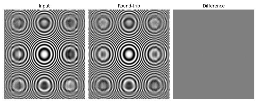
To begin with consider the same input of the first tutorial of the curvelets library. However, we will use here the PyLops operator to apply the 2D UDCT. A round-trip (i.e., forward-adjoing) is performed and the output is shown to be equal to the input, meaning that the adjoint of this transform is also the inverse.

shape = (256, 256)
x = make_zone_plate(shape)

Cop = pylops.signalprocessing.UDCT(shape)

y = Cop @ x
xinv = Cop.H @ y

fig, axs = plt.subplots(1, 3, figsize=(10, 4))
axs[0].imshow(x, cmap="gray", vmin=-1, vmax=1)
axs[0].set_title("Input")
axs[1].imshow(xinv, cmap="gray", vmin=-1, vmax=1)
axs[1].set_title("Round-trip")
axs[2].imshow(x - xinv, cmap="gray", vmin=-1, vmax=1)
axs[2].set_title("Difference")
for ax in axs:
    ax.axis("tight")
    ax.axis("off")
fig.tight_layout()

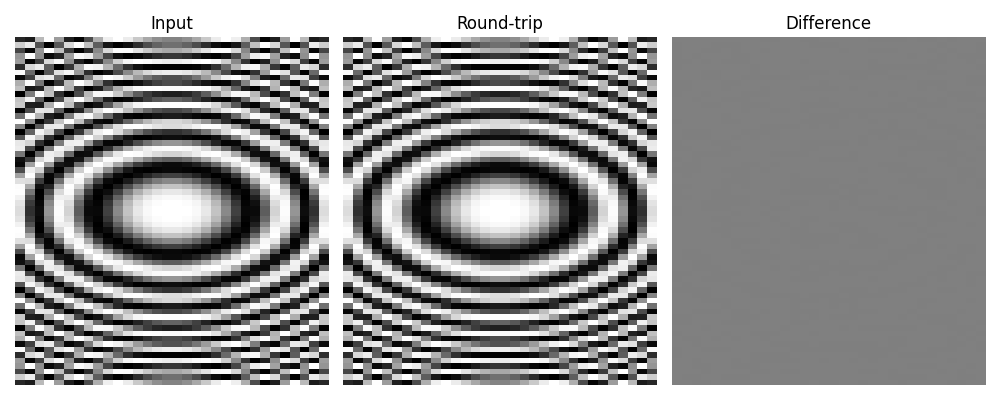
Next, the 2D version of the UDCT can also be applied along the last two axes of a N-dimensional input. This can be easily done with the aid of the pylops.Kronecker operator.

shape = (2, 3, 64, 32)
x = make_zone_plate(shape[2:])

# replicate over the first two axes.
x = np.tile(x[None, None], (shape[0], shape[1], 1, 1))

Cop = pylops.signalprocessing.UDCT(dims=shape[2:])
Iop = pylops.Identity(prod(shape[:2]))
Cop = pylops.Kronecker(Iop, Cop)

y = Cop @ x.ravel()
xinv = (Cop.H @ y).reshape(shape)

fig, axs = plt.subplots(1, 3, figsize=(10, 4))
axs[0].imshow(np.mean(x, axis=(0, 1)), cmap="gray", vmin=-1, vmax=1)
axs[0].set_title("Input")
axs[1].imshow(np.mean(xinv, axis=(0, 1)), cmap="gray", vmin=-1, vmax=1)
axs[1].set_title("Round-trip")
axs[2].imshow(
    np.mean(x, axis=(0, 1)) - np.mean(xinv, axis=(0, 1)), cmap="gray", vmin=-1, vmax=1
)
axs[2].set_title("Difference")
for ax in axs:
    ax.axis("tight")
    ax.axis("off")
fig.tight_layout()

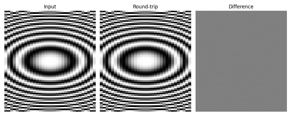
And similarly, if we want to apply the UDCT over any two axes, the pylops.Transpose can be used to re-organize the axes of the input prior to applying the transform

shape = (2, 64, 3, 32)
x = make_zone_plate((shape[1], shape[3]))

# replicate over the first two axes.
x = np.tile(x[None, :, None], (shape[0], 1, shape[2], 1))

Cop = pylops.signalprocessing.UDCT(dims=(shape[1], shape[3]))
Top = pylops.Transpose(shape, axes=(0, 2, 1, 3))
Iop = pylops.Identity(prod((shape[0], shape[2])))
Cop = pylops.Kronecker(Iop, Cop) @ Top

y = Cop @ x.ravel()
xinv = (Cop.H @ y).reshape(shape)

fig, axs = plt.subplots(1, 3, figsize=(10, 4))
axs[0].imshow(np.mean(x, axis=(0, 2)), cmap="gray", vmin=-1, vmax=1)
axs[0].set_title("Input")
axs[1].imshow(np.mean(xinv, axis=(0, 2)), cmap="gray", vmin=-1, vmax=1)
axs[1].set_title("Round-trip")
axs[2].imshow(
    np.mean(x, axis=(0, 2)) - np.mean(xinv, axis=(0, 2)), cmap="gray", vmin=-1, vmax=1
)
axs[2].set_title("Difference")
for ax in axs:
    ax.axis("tight")
    ax.axis("off")
fig.tight_layout()

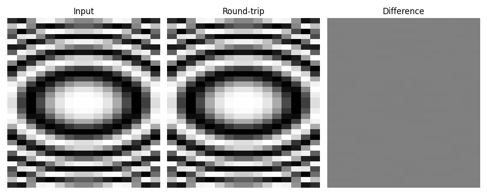
Finally, if the pylops.signalprocessing.UDCT is applied directly to a 3-dimensional (or N-dimensional) input, the 3D/ND version of the transform is used.

shape = (16, 32, 16)
x = make_zone_plate(shape[1:])

# replicate over the first axis.
x = np.tile(x[None], (shape[0], 1, 1))

Cop = pylops.signalprocessing.UDCT(dims=shape)

y = Cop @ x
xinv = Cop.H @ y

fig, axs = plt.subplots(1, 3, figsize=(10, 4))
axs[0].imshow(np.mean(x, axis=0), cmap="gray", vmin=-1, vmax=1)
axs[0].set_title("Input")
axs[1].imshow(np.mean(xinv, axis=0), cmap="gray", vmin=-1, vmax=1)
axs[1].set_title("Round-trip")
axs[2].imshow(np.mean(x, axis=0) - np.mean(xinv, axis=0), cmap="gray", vmin=-1, vmax=1)
axs[2].set_title("Difference")
for ax in axs:
    ax.axis("tight")
    ax.axis("off")
fig.tight_layout()