Downsampling

This example shows how to use the pylops.signalprocessing.Downsample2D operator to reduce the size of a 2-dimensional array along both of its directions.

Downsampling is performed in two steps: an anti-aliasing Gaussian filter is first applied to the input array, and the smoothed array is subsequently subsampled by the required decimation factors. Whilst a naive subsampling of the input array would fold any energy above the Nyquist wavenumber of the coarse grid back onto the retained wavenumbers (i.e., aliasing), the Gaussian filter removes such energy prior to decimation.

As the operator is linear, its adjoint (and, more interestingly, its inverse) can also be used to move back from the coarse to the fine grid; the latter represents a very simple form of super-resolution.

import matplotlib.pyplot as plt
import numpy as np
from scipy import datasets

import pylops

plt.close("all")
np.random.seed(0)

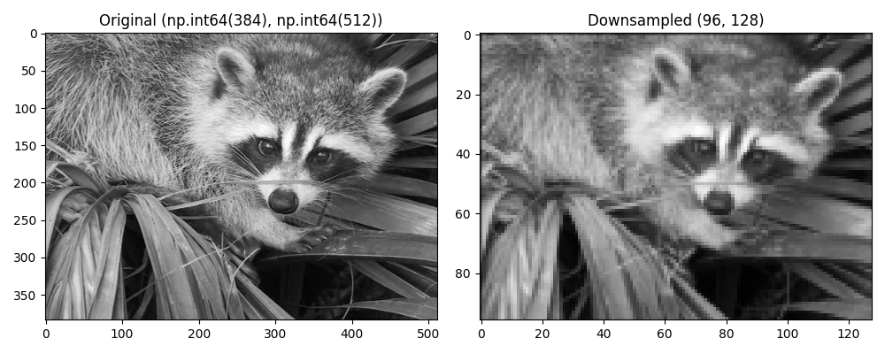
Let’s start by creating a 2-dimensional input vector containing an image from the scipy.datasets family and downsample it by a factor of 4 in both directions.

x = datasets.face()[::2, ::2, 0].astype(np.float64)
nz, nx = x.shape

Dop = pylops.signalprocessing.Downsample2D((nz, nx), factors=4)
y = Dop @ x

print(Dop)
print(f"Model size: {Dop.dims}, Data size: {Dop.dimsd}")

fig, axs = plt.subplots(1, 2, figsize=(10, 4))
axs[0].imshow(x, cmap="gray")
axs[0].set_title(f"Original {Dop.dims}")
axs[0].axis("tight")
axs[1].imshow(y, cmap="gray")
axs[1].set_title(f"Downsampled {Dop.dimsd}")
axs[1].axis("tight")
plt.tight_layout()

<12288x196608 Downsample2D with dtype=float64>
Model size: (np.int64(384), np.int64(512)), Data size: (96, 128)

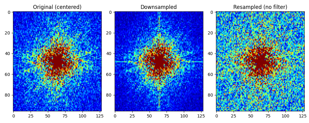
The role of the anti-aliasing Gaussian filter becomes evident if we take the input and output in the frequency domain. Note how a simple resampling of the input array (i.e., picking one every four samples in each direction) would lead to aliasing of the high wavenumbers, which is instead not present in the downsampled array.

Fop = pylops.signalprocessing.FFT2D((nz, nx), fftshift_after=True)
F1op = pylops.signalprocessing.FFT2D((nz // 4, nx // 4), fftshift_after=True)

xf = Fop @ x
yf = F1op @ y
yf1 = F1op @ x[::4, ::4]

fig, axs = plt.subplots(1, 3, figsize=(10, 4))
axs[0].imshow(
    np.abs(xf)[
        nz // 2 - nz // 8 : nz // 2 + nz // 8, nx // 2 - nx // 8 : nx // 2 + nx // 8
    ],
    cmap="jet",
    vmin=0,
    vmax=0.005 * np.abs(xf).max(),
)
axs[0].set_title("Original (centered)")
axs[0].axis("tight")
axs[1].imshow(np.abs(yf), cmap="jet", vmin=0, vmax=0.005 * np.abs(yf).max())
axs[1].set_title("Downsampled")
axs[1].axis("tight")
axs[2].imshow(np.abs(yf1), cmap="jet", vmin=0, vmax=0.005 * np.abs(yf1).max())
axs[2].set_title("Resampled (no filter)")
axs[2].axis("tight")
plt.tight_layout()

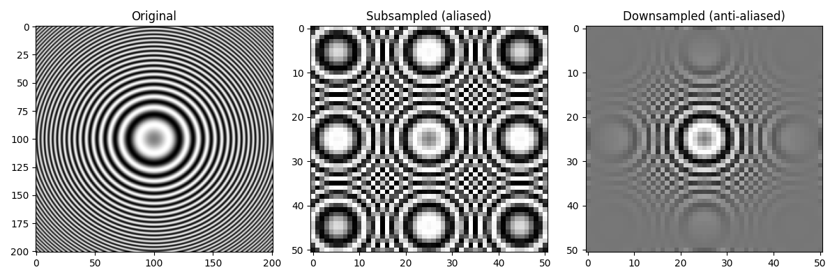
Similarly, if we take a synthetic image containing a rapidly oscillating pattern, where aliasing is easy to spot, we can see the difference between our downsampled image with the one obtained by simply picking one every four samples in each direction (which is equivalent to using sigma=0).

nz1, nx1 = 201, 201
iz, ix = np.meshgrid(np.arange(nz1), np.arange(nx1), indexing="ij")
xosc = np.sin(0.1 * np.sqrt((iz - nz1 // 2) ** 2 + (ix - nx1 // 2) ** 2) ** 2 / 10.0)

Dop = pylops.signalprocessing.Downsample2D((nz1, nx1), factors=4)
Dop_noaa = pylops.signalprocessing.Downsample2D((nz1, nx1), factors=4, sigma=0.0)

fig, axs = plt.subplots(1, 3, figsize=(12, 4))
axs[0].imshow(xosc, cmap="gray")
axs[0].set_title("Original")
axs[0].axis("tight")
axs[1].imshow(Dop_noaa @ xosc, cmap="gray")
axs[1].set_title("Subsampled (aliased)")
axs[1].axis("tight")
axs[2].imshow(Dop @ xosc, cmap="gray")
axs[2].set_title("Downsampled (anti-aliased)")
axs[2].axis("tight")
plt.tight_layout()

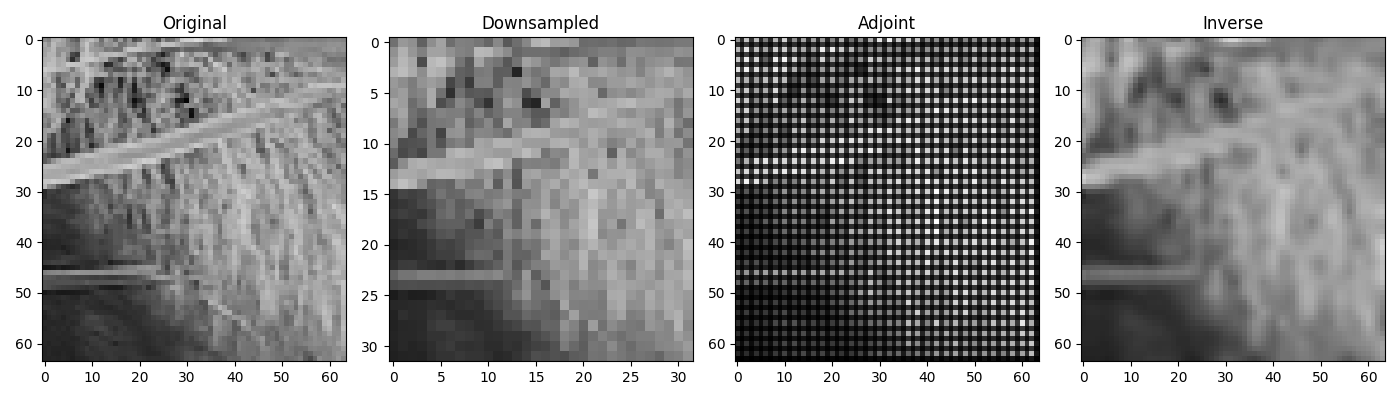
Finally, we consider the inverse problem: given the downsampled data, can we retrieve the original, finely sampled image? As the operator has many more columns than rows, this problem is heavily underdetermined and we must regularize it. Here we simply ask for a smooth solution by penalizing the Laplacian of the model. We compare the estimated model with the adjoint, which spreads each coarse sample back over the fine grid.

x = datasets.face()[400:528:2, 400:528:2, 0].astype(np.float64)
nz, nx = x.shape

Dop = pylops.signalprocessing.Downsample2D((nz, nx), factors=2)
y = Dop @ x

xadj = Dop.H @ y
D2op = pylops.Laplacian((nz, nx), weights=(1, 1), dtype="float64")
xinv = pylops.optimization.leastsquares.regularized_inversion(
    Dop, y.ravel(), [D2op], epsRs=[np.sqrt(0.1)], **dict(iter_lim=200)
)[0]
xinv = xinv.reshape(nz, nx)

fig, axs = plt.subplots(1, 4, figsize=(14, 4))
axs[0].imshow(x, cmap="gray", vmin=0, vmax=255)
axs[0].set_title("Original")
axs[0].axis("tight")
axs[1].imshow(y, cmap="gray", vmin=0, vmax=255)
axs[1].set_title("Downsampled")
axs[1].axis("tight")
axs[2].imshow(xadj, cmap="gray")
axs[2].set_title("Adjoint")
axs[2].axis("tight")
axs[3].imshow(xinv, cmap="gray", vmin=0, vmax=255)
axs[3].set_title("Inverse")
axs[3].axis("tight")
plt.tight_layout()